Will QE surprise on the upside or the downside?
The European Central Bank has practically communicated that it will decide on Quantitative Easing (QE) in its 22nd of January meeting, even if it is likely that Draghi will have again recourse to his salami communication tactics, whereby he first announces the decision in principle and then gives the detail. Still, one hopes the process will not be as extenuatingly long as the one followed for the purchase of Asset Backed Securities, as the market is not likely to be so patient this time.
In any case, since market expectations are concentrating more and more on a QE announcement, it is useful to analyse two aspects that could have a significant impact on market reactions at announcement:
- To what extent is QE already incorporated into financial prices, specifically €-area government bond yields?
- What are the specific modalities of QE that could determine its overall effectiveness?
In particular it is interesting to assess the risk that the ECB would either surprise on the upside, or on the downside, leading to lower, or higher, bond yields and also a lower, or a higher, € exchange rate.
Let´s examine the two aspects in turn.
As regards the first point mentioned above, possibly the easiest way to assess to what extent QE is already priced in is to start from the yield spread between peripheral and core bonds. Taking the two largest markets in the two categories, this means concentrating on the BTP-Bund spread and making assumptions about the variables entering the following equation. Indeed the current spread can be factored as follows:
c=ƒ-ϒSP
where:
c is the current spread
f is the value of the spread that would prevail if there was no expectation of QE (call it the fair spread)
S is the expected size of QE
γ is the impact of 100 billion of QE purchases on the BTP-Bund spread
and
P is the probability of QE.
Clearly, given the equation above, one can obtain P, given c, to be observed in the market, and assumptions about f, S and γ. Indeed one can obtain any of the four factors on the right side of the equation given the other three.
Chart 1 reproduces the yield on BTPs and Bunds, and the spread between the two, which is our point of departure to estimate the degree to which QE is already priced in.
Chart 1. BTP vs Bund yields (upper panel) and spread (lower panel).

Source: Bloomberg
Some assumptions about the possible values of the parameters of the equation above are reproduced in table 1:
Table 1. Decomposing the BTP-Bund spread
| Low impact | Intermediate impact | High impact | |
| Current Spread= c | 138 bp | 138 bp | 138 bp |
| Fair value= f | 180 bp | 180bp | 180 bp |
| Size of QE= S | 500 bn | 500 bn | 500 bn |
| Effect of QE per 100 bln. =ϒ | 5bp | 10 bp | 15 bp |
| Probability of QE = P | 1.68 | 0.84 | 0.42 |
Source: Authors’ calculations
In the table, depending on the assumed value of γ, i.e. the impact on the spread of a purchase of 100 billion €, the probability of QE incorporated into the current spread moves from (a nonsensical) more than 100% to a high probability of 84% for an intermediate value of the impact to a probability of 42% for a high value of the impact.
Of course, one can play with different values also for the other variables in the table to get different results. To give an idea of the possible combinations between the different factors, in Chart 1 we put on the horizontal axis different assumptions for S, the size of QE, gradually increasing from 200 to 1.000 billion. On the vertical axis we put the implied probability of QE. The 5 curves reflect different assumptions for γ, i.e. the impact on the BPT-Bund spread of 100 billion of QE purchases, from 8 to 16 basis points. In the chart we see that the probability implicit in the current spread goes down for both increasing values of γ and the assumed size of the purchases.
The chart and the table show that the conclusion about the degree to which QE is priced in the current spread depends on the chosen parameters. On the size, the central tendency of market expectations seems to be 500 billion €. On γ, i.e. the impact effect of 100 billion € of purchases, however, views are much more dispersed. One can start from the US experience with QE. The most relevant paper on this experience estimated a fall in the term premium in the Treasury market corresponding to approximately 2 to 5 basis point reduction per 100 billion $ of purchases. 1 In € terms, 100 € billion of purchases would, just taking literally the US experience, cause between 2.5 and 5.5 basis point yield reduction per 100 billion € of purchases. Estimates derived from investment bank publications for the €-area range widely, up to a maximum of 20 basis points.
If we concentrate on a size of 500 billion we should conclude, reading the result in Chart 1, that for all values of γ equal or lower than 12 basis points, which define the most plausible range of values, the current BTP-Bund spread prices in practically a 100 per cent probability of QE.
Chart 2. Different probabilities implied in the current BTP-Bund spread for different assumptions about the impact of 100 billion of QE purchases and about different sizes of the purchase program.
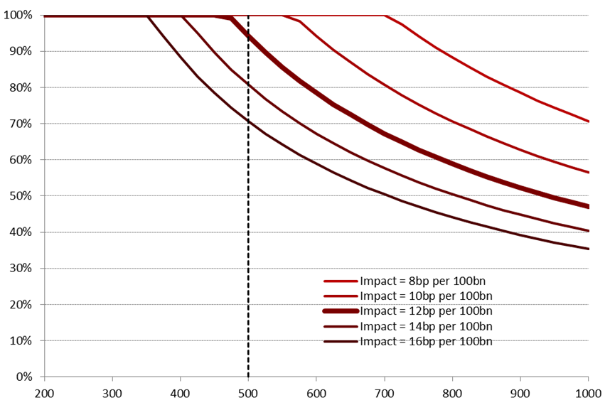
Source: Pictet Asset Management
To expand a little the exercise, one may wish to assess separately the effect on BTP and Bund yields. In order to do this we can follow two different approaches. A first approach assumes that the effect on BTPs relative to that on Bund is proportional to the ratio of the yield of the two bonds. This ratio was 2 to 1 at the beginning of 2014, thus the impact effect of QE on BTP yields should be twice as large as that on Bunds. This means that, for instance, if the BTP-Bund spread comes down by 5 basis points for 100 billion of purchases (i.e. γ= 5 bp) this would be due to a decrease of the BTP yield by 10 basis points and a reduction of the Bund yield by 5 basis point. A second approach is based on the idea that the search for yield means that, when the whole EMU yield curves’ structure moves lower, investors surrender the least yielding bonds in favour of those offering better returns. At the limit, this would imply that the entire reduction of the spread is due to lower BTP yield, with Bund yield remaining unchanged.
If we concentrate on a sensitivity (γ) of 12bp for 100bp and assuming that on Thursday the ECB announces a €500bn public QE, the 10Y BTP-Bund spread could settle at 120bp (180-12*5), only 3bp below where it is trading as we write, while in case of a larger €600bn QE (surprising a bit on the upside) the spread could fall by 15bp. Since expected money market rates ought to move higher for the distant maturities if QE is deemed credible, in the first case Bund yield to maturity may even rise a bit, while in the second it would fall but only by a few bp.
In all the reasoning above, the effect on yields derives from the compression of the term premium rather than of expected future rates, consistently with the results of Gagnon and al. referred to above and on the analysis of investment banks. What is still crucial is to split the yield effect between the real and the nominal component, in the hope that, as mentioned by Draghi, the effect would be mostly on the former component, which has more of an effect on the real economy and would indicate a move of inflation expectations back towards the level consistent with price stability. Our hunch here is that, based on anecdotal observation of the US QE experience, the entire reduction of nominal yields would be reflected in the real yield while inflation expectations would rise. Real yields as a result would move twice as much as nominal ones, in our interpretation.
As regards the second point mentioned at the beginning of this post, i.e. the characteristics that are likely to impact the overall effectiveness of QE, there are five of them that it is useful to consider one by one.
1. Risk sharing. There are two dimensions of risk sharing: first between the private sector and the Eurosystem; second, within the Eurosystem. As regards the first dimension, we assume the European Court of Justice (ECJ) Advocate General endorsement of a pari-passu credit status with reference to the OMT will be de facto applied to QE, unlike the Securities Market Program. The main reason is that a senior status would be disruptive for market valuations. We notice, however, that the application of the pari-passu clause to central banks is not straightforward. If indeed it was not possible to fully apply it, QE would lead to a situation where ‘loss given default’ would be shared among the residual bonds but not on the bonds ‘bought-back’ under QE. The theory says that the credit component of such bond yield has to rise in proportion to the size of the “buy back”. As an example, if under QE, €100bn of BTPs were bought, representing around 7% of Italy’s outstanding negotiable debt, so its CDS ought to rise in proportion. So on a 10Y BTP whose CDS is 194bp it would rise by around 14bp. In other words this would wipe out most of the QE impact on spreads even in case of a €600bn programme. As regards the second dimension, i.e. the distribution within the Eurosystem of the risk from the purchases, the question is whether the standard procedure will continue to apply, according to which risk on monetary policy operations is pooled, or whether risk will be apportioned to individual National Central Banks (NCBs), as suggested by Bundesbank President Weidmann. 2
Four considerations are relevant for this dimension. The first consideration is that, so far, the purchases of government securities by the ECB have resulted in hefty capital gains, as shown in a previous post. 3 With hindsight, the peripheral central banks should have insisted for keeping the risk on themselves, to avoid sharing with core central banks the large profits that eventually were generated. The second consideration relates to which kind of risk will be left with the relevant National Central Bank (NCB). While it would be technically straightforward to leave market and rating risk with the relevant NCB, there are strong limitations to the protection that a national central bank can give against the default of its government. Default by Treasury A, for example, would lead to severe financial stress also for NCB A, indeed most likely to negative equity, and the ability of a defaulted government to recapitalize its central bank is doubtful. Then the Target2 credit of the ECB, and indirectly of creditor NCBs, towards NCB A, now with negative equity, would have a much lower quality than a credit towards a well capitalized NCB. As a consequence risk will spill over to all other central banks in the system. This could be avoided only if a NCB could pledge external assets, say dollars, gold or future dividends to be distributed by the ECB, to the ECB, to protect it from possible losses. This would be analogous to the “settling” of Target2 balances by means of external assets, like dollars or gold, proposed by Sinn and would similarly impact the solidity of monetary union, as explained by Cour-Thimann and Papadia. 4 Indeed this would be a nice return to the 1970’s, when Banca d´Italia had to pledge gold to the Bundesbank in order to borrow international reserves. The third consideration, going in the opposite direction, is that a hybrid setup (which has a more than 50% probability, reading different leaks reported in the press), where risk is partially pooled may represent the price to be paid for a broader consensus (or less vocal opposition) on QE from the ECB hawks. The fourth consideration, also against risk pooling, is that it is somewhat unfair that creditor countries, which managed to maintain a better credit through sound fiscal policies, should now support the less prudent policies of some other members of the €-area in a risk pooling not explicitly decided by elected governments. In conclusion, keeping default risk with NCBs is technically difficult and will inevitably carry a negative message for the solidity of the €-area, but one may consider it a price to be paid to achieve higher consensus and deal with the “unfairness” of risk-pooling outside of an explicit policy choice.
2. Size. The second important characteristic of QE would be its size. As argued above, a size of 500 billion would, more or less, meet market expectations, a lower amount would likely disappoint it, a higher size would impress on the market the willingness of the ECB to really regain price stability. Of course, the strongest solution would be an open program that would continue until the Governing Council was satisfied that sufficient progress had been attained towards reaching the “lower but close to 2%” objective for price stability. It is unlikely, however, that the ECB will decide for such an approach just because of its open-ended nature, which caused already problems with the German Bundesverfassungsgericht (German Constitutional Court). The recent legal argumentation by the General Advocate of the ECJ, however, could encourage the ECB to go somewhat in that direction. For instance it could say that a certain amount of securities would be bought every month, say 40 or 50 billion €, for at least 12 months and that the Governing Council would review the progress achieved towards price stability after one year.
3. Composition of QE by asset class. The third important characteristic is the composition of the purchases per asset class. While the presence or absence of non-sovereign bonds would be of limited significance, still supranational and corporate bonds for 20-25% of the total size are a possibility. However, two other factors are more important here: the maturity of the bonds to be purchased and whether also inflation linked securities would be bought. As far as the maturity of the bonds is concerned, the main channel through which QE impacts on yields is through the portfolio balance effect, which is stronger the longer is the maturity of the purchased assets. So, for instance, purchases limited to the 1 to 3 year maturity, as in the OMT, would be much less effective than purchases in the medium to long-term bucket. The recent ECJ’s Advocate General opinion, implicitly asking for non-distortionary ECB measures, has implications also for the maturity mix of QE, forcing to extend its range, especially in case of a large amount. In fact the ECB ought to refrain from buying more than 25% at most of each issue. This is important for liquidity purposes, in order to leave enough bonds for healthy trading, but will also be important taking into account Collective Action Clauses (CACs). In fact, settlement agreements with the issuer become binding with the participation of 75% of bondholders and if the Eurosystem held more than this share this would become and impediment to possible rescheduling or haircut, since the ECB has rightly clarified that it cannot be part of a voluntary rescheduling. In conclusion, in order not to be distortionary, the ECB should buy no more (and to be on the safe side substantially less) than ¼ of each outstanding bond issue: we assume the optimal cap to be 20%. The following table shows the amount of EMU negotiable government bonds outstanding in different curve segments assuming an issue cap of 20%. It is clear that a €500bn program could be accommodated staying in the 3-10Y maturities, but if the size would reach €750 bn, purchases would have to extend to the 15Y maturities.
Table 2. Theoretical maximum QE size as a function of maturities (EUR bn) with a 20% cap.
|
Cap on CAC and non-CAC bonds 0.20 |
Target Maturity | ||
| 3Y-10Y | 2Y-15Y | 1Y-30Y | |
| 558 | 778 | 1044 | |
Source: JPMorgan
On the inclusion of index linked bonds, given that the purpose of QE is to lower the real rate, to provide economic stimulus and move inflationary expectations towards the 2.0% level, it is obvious that also inflation linked bonds, which are available in the largest jurisdictions of the € area, should be bought.
4. Composition of QE by jurisdiction. On this point, while choosing the ECB capital key or a key derived from the outstanding amounts of public bonds of the different €-area countries would likely not make much difference, the possibility, raised by Bundesbank President Weidmann and mentioned in some leaks about ECB deliberations, that only AAA sovereign bonds would be purchased under the QE program would have much more dramatic effects. This would mean buying only the securities of Germany, Luxembourg, the Netherlands, Finland and Austria. The total key in the ECB capital of these countries amount to 36% of the total.
The advantage of this choice would be that the risk of ECB purchases would be lower, at least as conventionally measured. 5
However the disadvantages would be far higher:
- As also recognized by ECB Board Member Peter Praet, the effect of QE on a composite €-area yield would be much lower (in the approach used in the first part of this post, γ would be lower) given that it would only directly impact about one third of the total market and the part that has the lowest yields, which has less room for further compression; 6
- QE is not expected to have macroeconomic effects because of increasing bank reserves, whereby the increase in base money would, through the multiplier, increase money supply and thus prices. Also based on the US experience, QE is expected to work mostly through its impact on bond yields and on the exchange rate, because of a portfolio balance and expectation effect;
- An AAA QE would aggravate rather than attenuate the perverse situation whereby interest rates are higher in the jurisdictions with worse macroeconomic conditions (the periphery) than in those with a better situation (the core);
- Concentrating QE on AAA countries would aggravate financial stability risks. Compressing even further the yield on core bonds would further push investors to “chase for yield”. For example, the Bundesbank has expressed some fears that very low yields are feeding a real estate bubble in Germany and further compressing the yield on German securities would aggravate this risk;
- The complaints of savers in core countries that they are “expropriated” by the ECB because of too low yields would become even more vocal.
- Sub-Investment grade countries ought to be eligible only if complying with a macroeconomic programme, as is the case for repo collateral. This would both abide with existing rules and at the same time entail an objective incentive for Greece to negotiate.
5. Degree of consensus around QE. Of course the higher would be the degree of consensus with which the Governing Council would reach its decision on QE the more effective would be the program. But, as already mentioned above, there are some trade-offs between different characteristics of a QE program. This applies in particular to the degree of consensus within the Governing Council for a QE decision. For instance if there was an attempt to keep risk with NCBs or limit the purchased securities to the medium part of the curve, the consensus in the Governing Council could be higher but the effectiveness of QE lower. But the issue of trade-offs applies also to other characteristics, for instance between the size of QE and its extension also to peripheral bonds, not only AAA securities.
Conclusions
The overall conclusion of this post is that a ‘consensual’ €500 bn QE is to a large extent already priced in current yields and, arguably, in the exchange rate. The relevant issue, from a market and policy point of view, is whether the actual ECB announcement will surprise on the upside or the downside with respect to this expectation. Five parameters that will determine the “strength” of the announced QE have been examined in this post: Risk sharing, Size, Composition by asset class, Composition by jurisdiction, Degree of consensus around the decision.
Concluding whether a positive surprise is more or less likely than a negative one is everybody`s guess, also because there are extensive trade-offs between the different characteristics and a better outcome on one aspect may be offset by a worse outcome on another one and vice versa In addition, the overall design might not be immediately clear on all technical aspects. Still, looking at the different leaks about the difficulty of the decision in the Governing Council, one cannot exclude market disappointment when eventually QE will be announced.
Nevertheless, a more constructive reading is possible if the compromise solution on the technical characteristics would allow the ECB to approve its purchase program with a broader support than recent ECB squabbles foretell. This and the connected expectation that the program could be continued until the desired price stability objective was regained could turn out to be the decisive factor in fostering a positive market reaction, especially considering that most other Central Banks have delivered sequential QEs. This possibility would certainly be perceived to be higher if the first delivery does not consume most ‘political capital’. We know from the “whatever it takes” pledge that political determination matters more than technical aspects (given market positioning).
This post was written jointly by Andrea Delitala of Pictet Asset Management and Francesco Papadia, with the assistance of Madalina Norocea.
- Joseph Gagnon, Matthew Raskin, Julie Remache, and Brian Sack in “Large-Scale Asset Purchases by the Federal Reserve: Did They Work?”, FRBNY Economic Policy review, May 2011[↩]
- See on the risk pooling, Guntram Wolff in Bruegel, Sovereign QE and national central banks – leaving national central banks to carry the default risk is impossible and dangerous, January 2015; The only known case of non pooling of risk for monetary policy operations was that of the so called „additional bank loans“ i.e. of bank loans that do not have the necessary characteristics to be used all across the € area and are used as collateral only with the national central banks accepting them at their own risk. It is particularly significant that risk pooling was also applied during the Securities Market Program, when arguably the risk of purchasing peripheral bonds was much higher than now [↩]
- Trust in Europe paid handsomely! [↩]
- Hans-Werner Sinn, Timo Wollmershaeuser, Target Loans, Current Account Balances and Capital Flows: The ECB’s Rescue Facility, CESifo Working Paper, No. 3500, November 2011; Francesco Papadia, Operational Aspects of a Hypothetical Demise of the Euro, Journal of Common Market Studies Volume 52, Issue 5, pages 1090–1102, September 2014 [↩]
- By conventional measure it is understood here that the same risk measurement used by private institutions would be used by the central bank. The economic fallacy of this approach was shown by Ulrich Bindseil and Juliusz Jabłecki in Central bank liquidity provision, risk taking and economic efficiency, ECB Working Paper Series, May 2013, showing that the risk taken by the central bank is endogenous to its actions and thus cannot be measured and managed as a private institution would do.[↩]
- “If we buy an asset in an impaired market with a high liquidity premium, the direct effect on the financial conditions will be much bigger compared with buying only safe AAA assets in well-functioning markets. If ultimately it was decided only to buy very safe assets it would be clear that the appropriate size should be greater. There are trade-offs.” Interview with Börsen-Zeitung, December 2014.[↩]
