Three macroeconomic issues and Covid-19
COVID-19 raises a number of serious issues of a sanitary, social and economic nature. While recognising the difficulty of giving definitive answers at this early stage, we attempt to shed light on three critical macroeconomic topics, to learn something about the economic consequences of the virus:
- What is the balance between the negative aggregate supply and demand effects of the COVID-19 shock?
- What will be the effect on the stock market of lower expected growth and greater uncertainty about future growth?
- Do we see signs of an impact on credit supply in Italy, the European country currently most affected by the virus?
Supply and demand and the COVID-19 shock
COVID-19 has had clear supply effects: quarantines, closed factories, supply chain disruptions and impaired mobility obviously affect production.1 The effects on demand are more difficult to gauge but it is critical from an economic policy point of view to get a sense of them because we have more confidence about how to deal with demand (through monetary and fiscal tools) than with supply deficiencies.
Changes in real goods prices can indicate whether COVID-19 is causing major demand effects. Specifically, if aggregate supply effects dominate demand effects, we should see prices going up as activity goes down, in a kind of repeat of the stagflation of the 1970s. At that time, central banks were in a dilemma about whether to increase rates to fight inflation or to reduce rates to support economic activity. If prices remain largely unchanged, we can conclude that aggregate demand has also been substantially negatively affected by the spread of the virus.
Of course, relevant consumer price index information will not be available for a number of months because of statistical and economic lags. The only timely substitutes are raw material prices and breakeven inflation expectations.
The idea underlying Figures 1 and 2 is that between 20 February and 28 February (the shaded area in the figures) markets were hit by a COVID-19 shock. Subsequently the global economy was hit by other shocks. In particular, on 28 February, the Fed chair said the Fed would act as appropriate, followed on 3 March by a 50 basis points rate cut. Also on 3 March G7 ministers pledged to “use all appropriate policy tools” to deal with the shock. Subsequently, a dispute broke out between Saudi Arabia and Russia over oil, and emergency measures to contain COVID-19 were extended to the whole of Italy. We can consider what happened in the six days highlighted in Figures 1 and 2 as the pure impact of the COVID-19 shock and as a kind of natural experiment from which to draw conclusions on its macroeconomic consequences.
Figure 1 reports all variables as indices (3 February =100). The variables are the Chicago Board Options Exchange’s Volatility Index (VIX), as a measure of stock exchange volatility, a global stock index and raw materials price indicators.
Figure 1 shows the thoroughly discussed impact of COVID-19 on VIX, which more than doubled, and on global stocks, which recorded losses of about 10%. We don’t find, however, any trace of emerging higher inflation in raw material prices. If anything, it seems that the effect of the COVID-19 shock on raw material prices has been negative, in particular for energy and agricultural products.
Figure 1: The COVID-19 shock: indices of stocks, VIX and raw materials prices
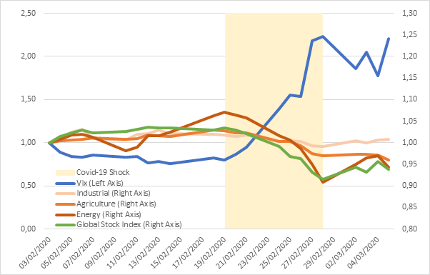
Source: Bruegel. Note: Agriculture includes unweighted average of corn, wheat, soybean, cocoa, sugar, rubber, ethanol; Energy: unweighted average of crude oil and natural gas; Industrial: unweighted average of copper, aluminum, zinc and tin; Global stock index is MSCI All-Country World Equity Index.
Figure 2 follows the same design and reports VIX and a global stock index, together with breakeven inflation in the United States and the euro area. In this figure the evidence is even clearer that the shock led to a reduction in expected inflation, as measured by break-even inflation, both in the US and in the euro area (by some 20-30 basis points).
Figure 2: The COVID-19 shock: indices of stock exchange, VIX and break-even inflation
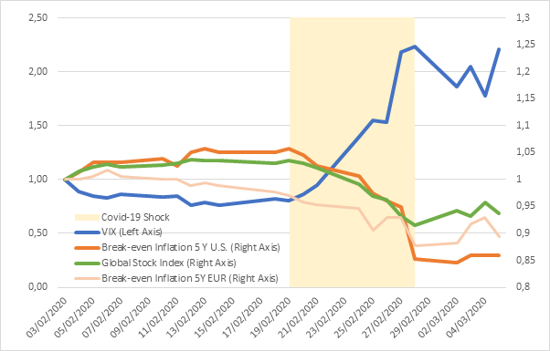
Source: Bruegel.
Figures 1 and 2 provide limited evidence but nevertheless indicate that the shock had significant demand-reducing effects. One cannot exclude that COVID-19 had even stronger effects on demand than on supply. Therefore, it makes sense to support demand. This does not settle, however, the subtler question of what would be the right mix of fiscal and monetary policy.2 Nor does it indicate whether, within the monetary policy tools, a reduction in interest rates would be the most appropriate move, given the specific features of the COVID-19 shock. In assessing fiscal policy, it should also be considered that additional expenses might not have much to do with aggregate demand but rather with the need to protect and support the population hit by COVID-19.
The impact of lower expected growth on shares
Data is lacking to assess the impact of uncertainty about growth, caused by COVID-19, on share prices. But the issue can be neatly considered in conceptual terms. Figure 3 shows hypothetical frequency distributions of expected growth rates.
Figure 3: Hypothetical distributions of expected growth rates

Distribution 1 is assumed to have prevailed before 20 February, ie before COVID-19, with higher growth/lower dispersion than the other three distributions. Distribution 2 is what would result if COVID-19 had only caused a higher variance in growth expectations with the same mean (mean preserving spread). Under a risk-aversion hypothesis, this should have a negative impact on financial variables including the stock market. Distribution 3 is what would result if the only consequence of COVID-19 was lower expected growth. Distribution 4 is, in all likelihood, what has actually happened, as the COVID-19 shock has brought down average expected growth but has also caused its variance to increase – a double whammy to growth expectations. Provided average expected growth does not change, as new information about the spread and the consequences of the virus becomes available, uncertainty should reduce and over time the distribution of growth expectations should move from distribution 4 to distribution 3. Reduced uncertainty about growth should bring about some recovery of the stock market. This would help reduce the apparent disproportion between the very deep fall of global stock prices, of more than 10% between 20-28 February, and any reasonable estimate of the actual damage to the global economy from COVID-19.
Finding empirical support for this argument is not easy but two contiguous issues can be documented:
- The increase in stock market uncertainty, as measured by VIX, from about 15 on 20 February to about 40 on 28 February (Figure 4);
- The fact that increasing uncertainty is negatively associated with losses on the stock market3 as seen in Figure 5, which reports the long-term level of VIX and US stock prices (SP 500), showing the negative correlation between the two variables, estimated at about 70%-75%.
Figure 4: VIX, 4 February to 5 March
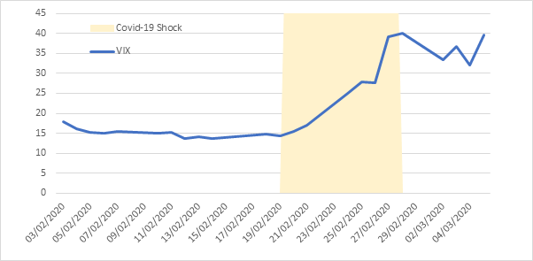
Source: Bruegel.
Figure 5: VIX and SP 500, January 1990 to March 2020
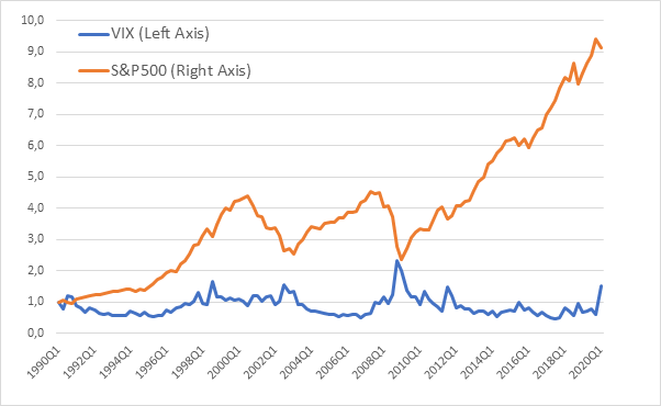
Source: Bruegel. Note: quarterly data.
Are there signs of an impact on credit supply in Italy?
Italy’s high debt, its long-term stagnation and a banking system that is still dealing with the legacy of the financial crisis, combined with the highest concentration of coronavirus in Europe, makes the country’s situation a very delicate one. A critical issue is whether there will be negative bank credit developments.
Of course, clear signs of credit supply deficiencies could only appear some months from now, when evidence about credit growth and credit conditions, as well as ratings, will start reflecting the effects of the spread of the virus. In terms of advance warning, one can look at the credit default swaps of large Italian companies. The mechanism that could lead to credit problems could be the higher default risk of firms borrowing from banks, which would impair the flow of bank credit.
Figure 6: Credit default swaps of selected Italian companies, 4 February to 5 March

Source: Bruegel.
Figure 6 shows an initial fairly strong increase in CDS for the selected non-bank firms as an impact of COVID-19, but then a significant recovery, so that by 28 February, the CDS are at a not much higher level than on the 20 February. Of course, this evidence does not say anything about the credit risk posed by small and medium size enterprises, which are predominant in the Italian economy.
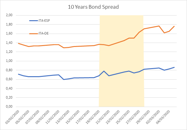
Additional, and more general, information about the credit risk posed by Italian private borrowers, albeit not very precise, can be derived from changes in the spread between Italian government bonds and those of other countries. The most revealing is the spread between Italian and Spanish bonds, since the often-used Italian-German bond spread is biased upwards by the flight-to-safety dynamic that is specific to Bund securities. The spread between the yield of Italian and Spanish securities conveys information on the overall risk posed by Italian private borrowers because the Italian state is a preferred creditor in Italy and the cost of its borrowing establishes a ceiling for private borrowers.
Figure 7: Spread between Italian 10-year bonds and German and Spanish securities, 4 February to 3 March
Source: Bruegel.
By this measure, the deterioration is limited to a few basis points. Much of the deterioration in the Italian treasury bond to Bund spread is shared with Spanish bonds, indicating that the specific Italian component is limited.
In conclusion, three messages can be drawn out from our assessment of the short-term impact of COVID-19:
- Aggregate demand effects from the shock are at least as important as aggregate supply effects, and thus demand-enhancing policies are justified;
- The stock market has been hit by both a deterioration in average expected growth and greater uncertainty, though the latter effect should dissipate over time;
- The impact on the credit risk posed by Italian borrowers seems to be, for the time being, limited.
- See M. Demertzis and G. Masllorens, ‘The cost of coronavirus in terms of interrupted global value chains’, Bruegel Blog, 9 March 2020, available at https://www.bruegel.org/2020/03/the-cost-of-coronavirus-in-terms-of-interrupted-global-value-chains/.[↩]
- Alessandro Leipold forcefully made the point that it should be fiscal policy that should answer to the shock. See ‘Whatever it takes’ Why urgent fiscal policy action is key to Eurozone success’, The Lisbon Council, 9 March 2020. Vitor Constancio, in a 4 March Twitter thread, while agreeing that the brunt of the action must be taken by fiscal policy, argued that central banks have a role to play in ensuring appropriate liquidity.[↩]
- Evidence broadly related to the effect of uncertainty on stock market volatility can be derived from Baker et al (2016), which documents a correlation between an index of economic uncertainty and the volatility of the stock price of individual firms. See Baker, S.R., N. Bloom and S.J. Davis (2016) ‘Measuring Economic Policy Uncertainty’, The Quarterly Journal of Economics 131(4).[↩]