The day after QE

In a previous post, published on Tuesday the 20^{th  1}  we addressed two issues:

1. Whether the expected Quantitative Easing (QE) of the European Central Bank was priced in bond yields, and in particular in the spread between Italian and German 10 year bonds (BTP-Bund spread);
2. Which were the characteristics to look at when the ECB would have announced its program to assess whether it would surprise upward or downward (risk sharing, size, composition by asset class, composition by jurisdiction and degree of consensus).

The announcement of Draghi on January 22^nd overall surprised on the upside, as market reactions showed. Looking at these reactions one cannot gather further information about the effects of QE. In addition, a comparison between our reading of market expectations and the QE announcement allows to “factor” the upside surprise into the various characteristics that we had identified in our post.

In this new post we first see what message market reactions sent about the effects of QE, then we examine how its characteristics compare with market expectations.

Market reactions and QE effectiveness.

 The market changes caused by the QE announcement can shed some light on the effect of QE. Indeed one element of uncertainty in assessing QE in our post was about the value of  γ, i.e. by how much the BTP-Bund spread would come down for 100 billion of QE purchases. The only conclusion we really felt confident about was that this would be equal or lower than 12 points. On how the spread reduction would be divided between the changes in the yield of BTPs and that on Bunds, we presented two cases: either the effect on the bund yield would be zero or it would be a half of that on the BTP yield.  In chart 1 we report the changes in the spread as well as in the yield in Italian, Spanish, German, French 10 year bonds and in the break-even inflation with a maturity of five year prevailing five year from now.

 Chart 1: Changes in bond yields, the BTP-Bund spread and inflation expectations

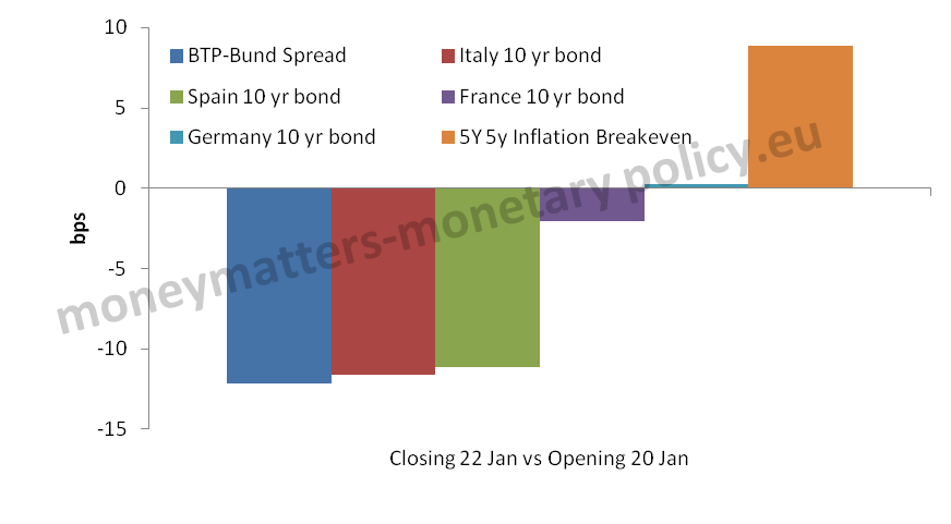
 Source: Bloomberg, Authors’ calculations

  In the spirit of an event study, here the window for the changes is measured in three days from the opening values on the morning of the 20^th to the closing of the 22^nd. Making the heroic assumption that the effect of QE was exhausted in the 3 days between the opening on the 20^th and the closing on the 22^nd, we should conclude that this is equal to about 4 points per 100 billion of purchases.  ² This figure is obtained by dividing the reduction of the BTP-Bund spread of 12 points in total by the additional purchases of government securities announced by Draghi, which we estimate at around 300-340 billion. This latter estimate is derived from subtracting from the 60 billion of purchases for 19 months (until September 2016) an extrapolation of 10 billion of monthly purchases of ABS and Covered bonds as well as 12 per cent of agencies purchases. This gives an amount of around 840 billion in total with respect to the 500 billion that we considered already priced in. At about 4 basis points, γ would be on the low side of the range that we considered as plausible in our previous post (3 to 12 bp per 100 billion of purchases). According to the impact effect, the 12 point reduction of the spread would derive entirely from a reduction of the BTP yield while the Bund yield would have remained unchanged. It should also be noted that break-even inflation increased by 14 basis points, so the sensitivity of inflationary expectations to 100 billion of QE would be also around 4 basis points. The fall of nominal yields and the increase in break-even inflation obviously meant a sizeable reduction in real yields. This was particularly sizeable on some bonds: for instance the yield on a long-term inflation linked BTP decreased by 20 basis points in two days.

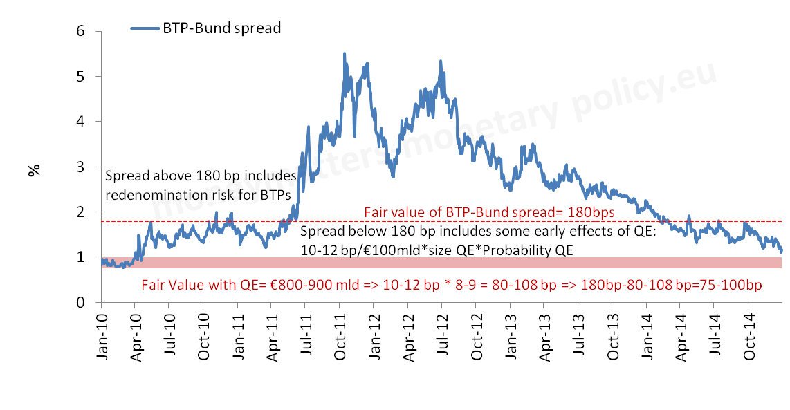
Of course, it is not granted that the entire effect of QE develops in just 3 days. Nor can one exclude, given Draghi`s announcement, that the size of government purchases would be higher than the 800-840 billion estimated above. So an alternative estimate for the effect of QE is presented in Chart 2. Here we have the actual BTP-Bund spread, a horizontal line for the value of 180 basis points we took as fair value for the spread in our previous post and assume a value of  of 10 or 12 basis points for γ and let the purchases of government bond reach up to a maximum of 900 billion. In this case the 10Y BTP-Bund spread would have a potential target of 100 to 75bp, so further below the current level.

Chart 2: BTP-Bund spread: current value, fair value and target value with additional QE effect. 

Source: Bloomberg, Pictet Asset Management 

A headwind to such further yield compression for peripheral bonds, however, comes from the default ‘risk segregation’ effect that, other things being equal, entails some negative repercussion on spreads. Further analysis is required on this point.

Let`s now examine here the different characteristics of the announced QE with respect to expectations.

Risk Sharing

This was clearly the most complicated aspect of the prospective QE. In order to address it we looked in our post at two different dimensions: first, the distribution of risk between the private sector and the Eurosystem, second the distribution of risk within the Eurosystem.

On the first dimension, Draghi confirmed our expectation that the ECB would not require senior status. He even reinforced this point by limiting the purchases of the Eurosystem to a maximum of 25% of each issue, so that the Eurosystem would not have a blocking minority for the possible application of Collective Action Clauses.

On the second dimension Draghi did not mention the fact, that we had underlined, that the Eurosystem has so far made quite some profits with its purchases of government securities (in the Securities Market Program). He spent, instead, quite some time illustrating the approach the ECB had decided about the distribution of risk within the Eurosystem, still trying to belittle its importance. As an important background consideration to this approach, he mentioned the difficulty, which we denoted as unfairness in our post, of redistributing risk among different countries in the €-area without an explicit political choice. Also to recognize this difficulty, he came out with a quite complex solution. Basically this solution says that 92 per cent of the risk of default risk on national securities should be borne by the relevant central bank. Of course Draghi did not explicitly talk about default risk, but this is the only relevant risk if the securities are held to maturity and not marked to market. He also mentioned that the risk on the 12% of securities from European Agencies will remain on the ECB, but of course the default risk of the EIB and similar agencies is minuscule and therefore it does not much matter whether this risk is shared or not. As we argued in our post, it is very difficult to avoid the risk of default spilling over to the entire Eurosystem from the default of one government and the relevant national central bank, if anything because of the tight financial linkages within the Eurosystem, in particular because of the Target2 balances. Still the overall solution is less forceful in the aspect of risk sharing than we expected. In particular the market may find it odd that the Eurosystem asks the market to bear a risk that it is not willing to bear itself. Still we accepted in our previous post that full risk-sharing was both unlikely and, to an extent, unfair

Size

The most visible upside in the actual QE announcement was on the size of the program. We argued in our previous post that 500 billion of purchases over one year were fully priced in but also that a somewhat higher amount was possible. Still we thought that the best solution of a “state dependent” open program that would tie the length of the program to progress on getting back to price stability, was unlikely. Actually we got 60 billion per month that, excluding an extrapolation of current purchases of Asset Backed Securities and Covered Bonds, would mean an increase of about 50 billion of new securities purchased every month. And the purchase program will last at least until September 2016 and possibly until “sustained adjustment in the path of inflation which is consistent with our aim of achieving inflation rates below, but close to, 2% over the medium term.” ( Mario Draghi, 22^nd of January 2015 Press Conference) will be achieved. Thus the program is quasi on and state contingent.

Composition by asset class

On the composition for asset class, in our post we emphasised that the longer the maturity the stronger would be the effect of the program, in particular because of the “portfolio balance effect”, but we limited our ambition to a maturity of 10 years. In addition we stressed the importance of also including inflation-protected bonds, to directly impact the real component of interest rates and thus bring inflationary expectations up towards the price stability objective of 2 per cent. The ECB announcement exceeded our expectations envisaging maturities up to 30 years, while including inflation-protected bonds.

Composition by jurisdiction

The choice to distribute purchases according to the ECB capital key was consistent with our, easy, forecast and dispelled our, albeit remote, fear that an AAA approach would be followed.

One aspect that was covered by the ECB announcement that we had not foreseen in our post was a maximum limit of 33 per cent per issuer. Indeed we thought that the limit per issue of 20-25 per cent, which we assumed, would make an issuer limit redundant. We had, however, not taken into account that the ECB already holds some government securities in its portfolio and that these, in the case of Greece, exceed the 33 per cent limit. And this provides an elegant way to avoid purchasing Greek bonds until when, some time in the Summer, the redemption of some bonds held by the ECB will reduce the ECB holdings below the 33 per cent level. It also allows some time to see what the results of the Syriza win in the Greek elections will mean for Greek bonds.

Degree of consensus

Another favourable surprise was on the degree of consensus with which the decision was taken. We do not know exactly how the voting went, but Draghi could report an important unanimous agreement on the fact that QE belongs to the legitimate tools of monetary policy. Just to reflect on the importance of this agreement, recall that this point of principle was widely debated in front of the German Constitutional Court on the occasion of the hearings about the Outright Monetary Transaction (OMT) program and that the Court had substantial doubts in this respect. Indeed a closer look would be warranted at the consistency between the position of the Bundesbank in front the German Constitutional court, against the OMT, and its agreement now that QE is a legitimate monetary policy tool. Draghi also reported a consensus (no explicit disagreement) on the specific risk sharing agreement reached and a “large majority” on the conclusion that now was the time to use that monetary policy tool that is QE.

In our post we had underlined that there existed trade-offs between the different characteristics of the program, in particular between risk sharing and the degree of consensus with which the decision was achieved. Overall, the combination of the quasi Solomonic approach achieved on risk sharing (of course Solomon proposed splitting the baby 50/50 and not 92/8) and the degree of consensus achieved on the QE decision looks favourable to us. This impression could be spoiled, however, by future loud complaints by the Council members who did not approve QE and attention will have to be devoted to this aspect. It is also important to note that Draghi reiterated that OMT is still there to deal with redenomination risk, if this were to reappear. So the Eurosystem has two tools to deal with two different problems: OMT for the idiosyncratic risk affecting one single country and QE as an aggregate monetary policy tool. This is also relevant for the risk discussion carried out above. Of course it should also be noted that the distribution of default risk depends on its probability and this is the joint probability of a country managing its fiscal situation in such an unsound way as to raise the probability of default and of the remedial action constituted by an ESM program reinforced by OMT not being sufficient to avoid default. A very small probability in our view.

In conclusion, the QE announcement had an impact effect on the BTP-Bund spread and on inflationary expectations of about 4 basis points per 100 billion of additional purchases with respect to expectations. One cannot exclude, however, that QE will continue to have an effect beyond its initial impact, further compressing bond yields, in particular of peripheral countries, and increasing break-even inflation. For instance, a BTP-Bund spread of 75 to 100 basis points could be reached in the most favourable scenario.

The increase in size, the quasi-open character, the very long maturity of the bonds to be bought and the higher degree of consensus are contributing the most to the upward surprise in the announcement of QE. The specific approach to risk sharing is less forceful than one could have hoped, but does not offset the positive factors mentioned above.

 This post was written jointly by Andrea Delitala of Pictet Asset Management and Francesco Papadia, with the assistance of Madalina Norocea.

1. Will QE surprise on the upside or the downside?[↩]
2. The assumption here is that in our post on the 20^th we captured whatever effect of QE was anticipated by the market at the time of writing; over the following days leaks about a possibly larger size and eventually the announcement of QE caused further market reactions.[↩]