Until when will the US and the €-area be awash with central bank liquidity?

 

If you are impatient, my tentative answer to the question in the title is: 2022 for the US and 2028 for the €-area, meaning that we can expect another 6 years of abundant central bank liquidity ¹ in the US and a dozen years in the €-area. If you bear with me a while longer, I can explain how I do reach this, I believe surprising, result and why it matters.

The history of central bank liquidity over the last decade or so in the US and the €-area, but also in other advanced economies like the UK, is very simple. Until the beginning of the Great Recession, both the Fed and the ECB gave to banks just the liquidity they needed to satisfy reserve requirements and autonomous factors. Basically they targeted zero excess liquidity. This set the policy rate, the Federal Funds Rate in the US and EONIA in the €-area, practically in the middle of the corridor between the absorbing (the bottom) and the providing (the ceiling) central bank liquidity facilities.

While sharing this fundamental analogy, the FED and the ECB frameworks were different in some respects. The most important difference was that the law did not allow the FED to pay interest on bank reserves, and thus the bottom of the corridor for the FED was necessarily at 0, while the ECB could remunerate reserves and thus could move the bottom together with the entire corridor.

The liquidity situation changed with the beginning of the Great Recession, particularly after the failure of Lehman Brothers: central banks reacted to the sudden evaporation of private liquidity, both in the form of market liquidity and funding liquidity, by providing a huge amount of central bank liquidity. In essence this is the phenomenon behind the literal explosion of FED and ECB balance sheets in October 2008, as seen in chart 1. The pattern is somewhat different and the increase is larger for the FED (by a factor of 5) than for the ECB (by a factor of less than 3). In addition the specific channels through which the FED and the ECB provided the large amount of liquidity leading to the balance sheet explosion were different. Still the similarities in the balance sheet developments between the two central banks are more important than the differences, including the fact that their total balance sheet remained very large, not getting back to some historic norm, for the successive 8 years.

Chart 1. Total central bank balance sheets.

 

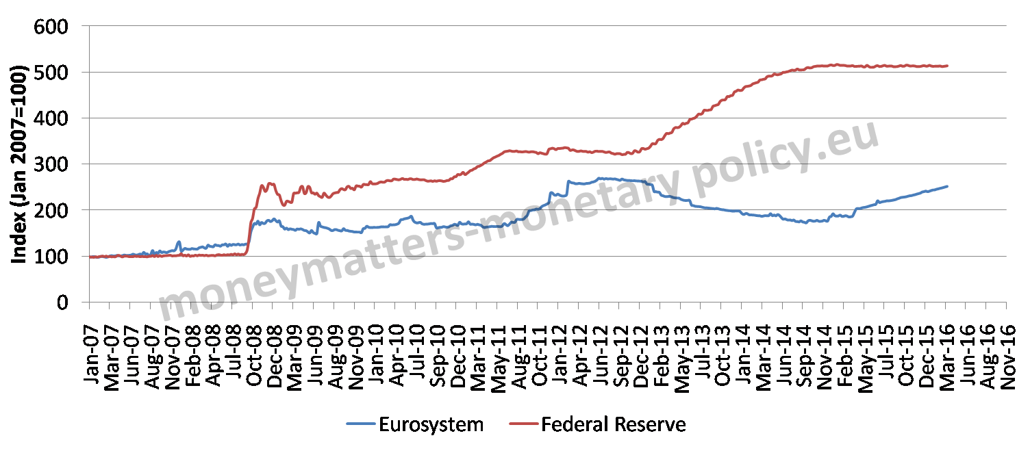
Source: ECB, FED

The huge increase of the balance sheet and the corresponding increase in bank reserves had two important implications for monetary policy, one theoretical and one operational. The theoretical implication is that it became untenable to maintain any Friedmanian notion of money multiplier: bank reserves (and with it base money) exploded but monetary aggregates remained very subdued for too long a period to continue believe that a constant, or at least forecastable, money multiplier is a stable parameter of the economy. The operational implication is that the central bank interest rate was progressively compressed towards the bottom of the corridor, i.e. the rate of the central bank deposit facility.

This is clearly seen in Chart 2, reporting the ECB interest rate corridor: while EONIA was close to the centre of the corridor in the pre-crisis area (shaded in light blue), it moved, albeit with a lot of volatility, to the lower part of the corridor in the first phase of the crisis (shaded in darker blue) and then it settled just close to the bottom in the last 5 years or so (darkest area).

Correspondingly, the most relevant policy rate became the one on the deposit facility, which defines the bottom of the corridor: banks were mostly interested about the rate at which they could deposit excess liquidity with the central bank, not about the cost of their recourse to lending facilities, which had become nearly redundant given the large amount of liquidity outstanding.

 

Chart 2. The ECB interest rate corridor*.

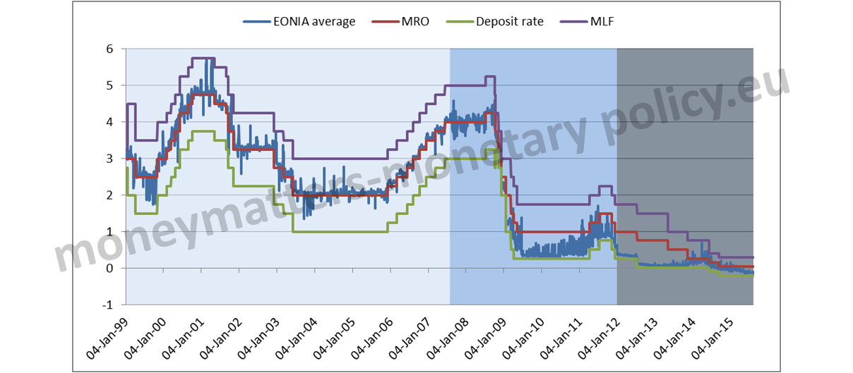
Source: ECB

 

* Eonia is the overnight rate, MRO is the rate on Main Refinancing Operations, Deposit rate is the rate of the ECB absorbing facility and MLF is the rate on Marginal Lending Facility, i.e. the rate of the ECB standing lending facility.

In central bank jargon, the approach for the central bank to steer interest rates moved from a balanced approach to a “floor approach”.

The question addressed in this post is for how long we can expect, on the basis of current information, this situation of abundant central bank liquidity to last and what its consequences are, for the control of interest rates by the central bank and for financial stability.

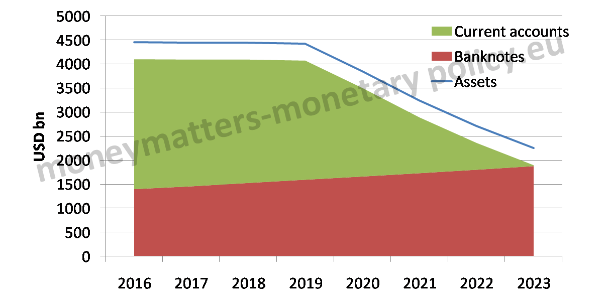
In chart 3 you find an extrapolation of the balance sheets, and in particular of liquidity, of the two central banks: the first panel is for the FED, the second for the ECB.

Chart 3. Extrapolation of the FED and ECB balance sheet.

 

FED

 

ECB

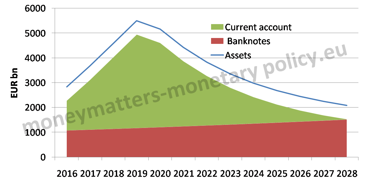
Source: ECB, FED

In the chart the linearly increasing reddish bottom area denotes the extrapolation of banknotes, the green area denotes current accounts, which is another name for central bank liquidity, the blue line represents the total size of the balance sheet and the difference between the blue line and the top of the green area represents “other liabilities”, i.e. those smaller liabilities items with no relevance for monetary policy. ²

In the FED chart you see that liquidity is extrapolated to remain exceptionally abundant, i.e. higher than 100 billion ³ until between 2022 and 2023. In the case of the ECB the extrapolation shows a return to “normality” only in 2028. This means that central bank liquidity will remain exceptionally large in the US for a total of around 15 years, in the €-area the period of exceptionally large liquidity will be around 20 years. The fact that central bank liquidity will remain so abundant for so long is an indication of the severity and long lasting effects of the Great Recession.

Indeed to find periods of so large increases of central bank balance sheets one has to go back to the two World Wars, as shown in the paper by Niall Ferguson, Andreas Schaab and Moritz Schularick ⁴. The indication that comes out of this comparison is that, from a monetary point of view, the Great Recession created the same stress as two catastrophes like the two world wars.

Of course, the assumptions used to extrapolate the balance sheet of the two central banks could turn out to be wrong, in particular because the two central banks may carry out much more active and early sales of securities than I assumed. Still the change in assumptions with respect to current expectations would need to be quite strong to substantially reduce the time horizon over which liquidity would return to normality.

At the beginning of this post I wrote that I would explain, first, how long the exceptionally abundant central bank liquidity situation would last and, second, why it matters. I hope I clarified the first point. Let me come now, very briefly, to the second one.

One first, obvious, consequence of the very abundant and persistent liquidity is that the “floor approach” to the steering of interest rates by the central bank is there to stay for quite a while longer. This approach would allow the central bank to raise its rate by increasing the bottom of the corridor but was not the one the ECB preferred until the Great Recession, as it was more comfortable in keeping the banks always in need of its liquidity. A floor approach is, however, an entirely legitimate way to steer rates. Ulrich Bindseil assessed it 5 years ago ⁵ as one of the possible approaches to interest rate control. In addition, it is my understanding that the FED is looking with interest at this approach as a permanent one in its study on the long-term monetary implementation framework. While feasible and not obviously undesirable, a floor approach is different from one in which liquidity conditions are kept balanced. For instance, in such an approach the width of the corridor is much less relevant and it makes no sense to say that the rate on refinancing operations is the “main” rate, as the ECB does.

Another clear consequence is that the short term money market is unlikely to regain the kind of depth and turnover it had before the Great Recession: if the central bank continues offering large amounts of liquidity, banks will probably have less of a need for an active market over which to exchange liquidity. An ancillary consequence is that the overnight interest rate loses much of its importance as an indicator of monetary conditions.

It is not easy to predict, instead, what would be the consequences for financial stability from a situation of persistent surplus of central bank liquidity. The fact is that there is hardly a precedent to this situation and it is thus very difficult to forecast its consequences, especially over the medium to long term. On one hand, the availability of large amount of central bank liquidity should avoid situations of liquidity stress. On the other hand, its persistence may give incentives to financial market participants to engage into unsound practices of the kind that led to the Great Recession. Personally, what bothers me is exactly that we do not know what the consequences could be.

In any case, unless the assumptions used to extrapolate the balance sheets of the two central banks turn out to be severely wrong and the FED and the ECB engage into an active program of selling of securities, there is still quite some time to decide whether a “floor approach” to interest rate steering by the central bank is desirable or not as a long lasting device and to ascertain what are the consequence of a very abundant and persistent provision of central bank liquidity.

This post was prepared with the assistance of Madalina Norocea.

 

Annex

Federal Reserve

The following balance sheet elements were considered:

Assets

• US Treasury securities
• Federal agency debt securities
• Central bank liquidity swaps
• MBS
• Repos&Loans
• Other assets
• Commercial paper funding facility
• Term auction credit

Liabilities

• Banknotes

First part of the exercise

Actual values were considered up until April 2016 for both assets and liabilities. Thereafter we extrapolated the asset side as follows:

• Until Jan 2019 all items were held constant at the current value, subsequently Treasuries were decreased by 20 billion each month until Dec 2020. Each year after that it was assumed that 15% of the stock of Treasuries was sold.
• Federal agency debt securities were considered constant until the end of the exercise.
• Central bank liquidity swaps, Repo&Loans, Commercial paper funding facility and the Term auction credit were kept at zero for the entire extrapolation.
• MBS were assumed to mature according to the weighted average duration of 6.5 years mentioned by the FED in the 2015 SOMA report.
• Other Assets were considered constant until the end of the exercise.

The total of these items represents the extrapolated total assets.

Second part of the exercise

• We take the extrapolated total assets of January of each year.
• We increase the value of Banknotes by the GDP growth rate in the below table.
• The difference between the two items gives the extrapolated current accounts.
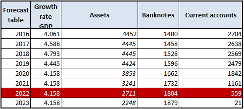
• The exercise ends in 2023 as the value of 100 billion of liquidity is reached between 2022 and that year.

Table Appendix 1. FED Extrapolated total assets, banknotes and current accounts.

 

 

European Central bank

The following balance sheet elements were considered:

Assets

• USD repo
• Net foreign assets
• Domestic assets
• MRO
• LTROs +TLTRO2
• MLF+FTO
• Policy portfolios

Liabilities

• Banknotes

First part of the exercise

the following assumptions were used:

• USD repo, Net foreign assets, Domestic assets, MRO and MLF+FTO are kept constant at the current values until the end of the exercise.
• LTROs and TLTRO2, as well as policy portfolios have been extrapolated as follows: for June 2016 we consider this account equal to 15% of the total long-term bank bond issuance. The value is maintained constant until Jan 2020. From then on it is fixed at 150 bn until the end of the exercise. This was the value for this item in 2007 prior to the crisis.
• For the policy portfolios:
  • Each month we account for 4 bn maturity under the old purchase programmes and new 80 bn purchases under the current purchase programme .
  • From Jan 2020 we account for 20% yearly selling of the outstanding stock while the 4 bn of monthly maturing securities continues.

The sum of the above mentioned items is the Total simplified assets

Second part of the exercise

• We take the extrapolated total assets of January of each year.
• We increase the value of Banknotes by a constant GDP growth rate (see table below).
• The difference between the two items gives the extrapolated current accounts.
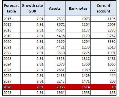
• The exercise ends in 2028.

 

Table Appendix 2. ECB Extrapolated total assets, banknotes and current accounts.

1. The terms central bank liquidity, bank reserves and banks current accounts with the central banks will be used interchangeably in this post. The adjacent concept of base money will also be occasionally used.[↩]
2. The rough assumptions to carry out the calculations are reported in annex. Basically two items dominate the balance sheets of the two central banks: securities bought under „QE“ programs on the asset side and banknotes on the liability side. Assumptions about these two items are critical for any extrapolation exercise.[↩]
3. This is the “normal” level assumed by the FED in its SOMA report for 2015 that also engaged into an extrapolation exercise similar, if more sophisticated, than the one reported in this post. The FED exercise sets at 2022 the year in which liquidity will reach its “normal” 100 billion size.[↩]
4. Central bank balance sheets: expansion and reduction since 1900, ECB Forum on Central Banking, May 2014, Monetary Policy in a changing Financial Landscape, Conference proceedings.[↩]
5. Theory of monetary policy implementation, in The Concrete Euro: Implementing Monetary Policy in the Euro Area, Paul Mercier and Francesco Papadia eds., Oxford University Press , 2011. [↩]