Measuring macroeconomic uncertainty during the euro’s lifetime
Together with Monika Grzegorczyk
1 Introduction
It has become a cliché in the publications of official economic institutions and the speeches of their leaders to lament exceptional uncertainty. The complaint is made so often that the adjective ‘exceptional’ cannot always be true. The complaint does, however, ring true currently, with the economic situation considered more uncertain than in the last 20 years. However, a solid empirical basis should be given to this view by properly measuring macroeconomic uncertainty. This is the purpose of this paper.
Research already shows the adverse effects of uncertainty on financial markets, household spending and overall economic activity (Gieseck and Rujin, 2020). Coibion et al (2021) showed that greater uncertainty makes households spend less. Bloom (2009) suggested that greater uncertainty causes firms to temporarily pause investment and hiring. Also, elevated risk premia lead to increased borrowing costs, together with the likely reduction in loan provision, which dampens investment even more (Gilchrist et al, 2014). The relationship between uncertainty and inequality is, however, ambiguous. While some research shows that uncertainty reduces inequality, this is due to lower investment and a higher risk premium that leads to the reduction of asset prices and therefore the of financial wealth of investors holding those assets (Theophilopoulou, 2021). The decline in inequality is thus not caused by improving the status of the worse off. In fact, uncertainty might be especially harmful to the poorer segments of society, which do not have room for more precaution in their consumption, credit and investment decisions (Ben-David et al, 2018).
While uncertainty cannot easily be reduced in relation to economic developments, uncertainty about economic policies can be reduced. Better communication between decision-makers and society is needed. As McMahon (2020) rightly pointed out: “uncertainty about policy is not the same as policy uncertainty”. Uncertainty about interest rates, quantitative easing programmes and details about the adjustment period contribute to lower investments and spending. Even if the inflationary component dominates, there is room to improve fiscal policies. For example, support programmes and tax adjustments introduced in response to increasing energy prices can be better targeted so that they do not have a negative effect on the price index (Sgaravatti et al, 2021).
To measure macroeconomic uncertainty and assess if it has really been exceptional, we need to define it precisely (see the Appendix for a formal definition). The basic idea is that observable forecasts of macroeconomic variables are transformations of the sets of macroeconomic information, which are so complex as to be unobservable, prevailing when the forecasts are made. Thus by observing how forecasts change over time we measure the flow of macroeconomic surprises, ie how developments differ from expectations. The more intense the flow of surprises, the greater uncertainty is.
Analogously, different forecasts among forecasters are evidence of uncertainty.
Our definition of uncertainty is precise, but also narrow and idiosyncratic. It makes no assumption about risk neutrality or aversion, and does not address the differences between risk, when a given frequency distribution is known, and radical uncertainty, when this is unknown. It also differs from volatility measures drawn from financial prices, such as the VIX Index for the US stock exchange, and the VSTOXX volatility benchmark for the European market, and from stress measures such as the ECB-estimated Composite Indicator of Sovereign Stress (CISS). It is also different from volatility, measured by the changes in the actual values of a given variable. Our definition corresponds, however, to the concept of uncertainty used in management literature (Bennett and Lemoine, 2014).
We translate our basic idea into four concrete indicators of macroeconomic uncertainty, measured over the lifetime of the euro:
- How the macroeconomic forecasts of a given institution for the same time period change over time;
- How the macroeconomic forecasts of a given institution deviate from realised outcomes (in other words, forecasting errors);
- How the macroeconomic forecasts of different institutions deviate from one other over a given time period;
- How dispersed the forecasts of different professionals are.
We also try to measure whether the ‘stag-‘ or the ‘-flationary’ component is strongest in the overall stagflationary shock caused by the Russian invasion of Ukraine. Finally, we check whether the return to the pattern before COVID-19, as documented by Grzegorczyk et al (2021), remains the prevailing view of forecasters.
Data sources and limitations
We use three data sources for the euro area: ECB staff macroeconomic projections, the ECB Survey of Professional Forecasters (SPF), both of which are published quarterly, and International Monetary Fund economic forecasts featured in the World Economic Outlook, published each spring and autumn. To deal with the problem that the forecasts are published at different times of the year, we take yearly averages.
While uncertainty is not directly observable, since it is related to subjective beliefs about the economy, its consequences can be observed. Our four indicators of economic uncertainty consist of deviations from past predictions, forecast errors and differences between forecasters. Bank of England (2013) research showed that the dispersion of annual GDP growth forecasts was the least correlated with the first principal component of uncertainty, implying that there are better measures than GDP dispersion to assess uncertainty, although none fully captures its effects. Aware of this shortcoming, we concentrated on two fundamental macro variables, inflation and GDP growth. There are some limitations to our method. Annual averages do not fully mitigate the effect of different frequencies of predictions, which implies that some forecasters will have an information advantage. This issue is especially pronounced in same year predictions (eg predictions done in different quarters of 2021 for the annual average in 2021). In the case of ECB staff projections, and the ECB’s Survey of Professional Forecasters (SPF), forecasters are asked in Q1, Q2, Q3 and Q4 what will be the average inflation rate in the same year. Naturally, their forecasting error decreases with every quarter. In the case of the IMF, the prediction is made twice a year for the yearly value of the same year. To assess the impact of this time difference, we measured the average forecast error of predictions for 1999-2021: the SPF error is lower by 0.1 percent and 0.2 percent for inflation, and 0.3 percent and 0.1 percent for GDP growth, compared to ECB and IMF, respectively. An additional limitation mentioned by the ECB (2022a) is that its working-day-adjustment of annual growth rates is different to that of the IMF.
2 Changes over time in forecasts from the same institution
In this section, we use changes in ECB, IMF and SPF forecasts over time to measure the level of uncertainty. We check how different the predictions for a given year are from those made one and two years previously year. For instance, we take an average of quarterly forecasts made in 2021 about 2021, and we compare them with those done in 2019 and 2020. To illustrate our procedure, we start with changes in the ECB projections.
Figure 1: Changes in ECB projections over time, inflation and GDP growth (percentage points difference)
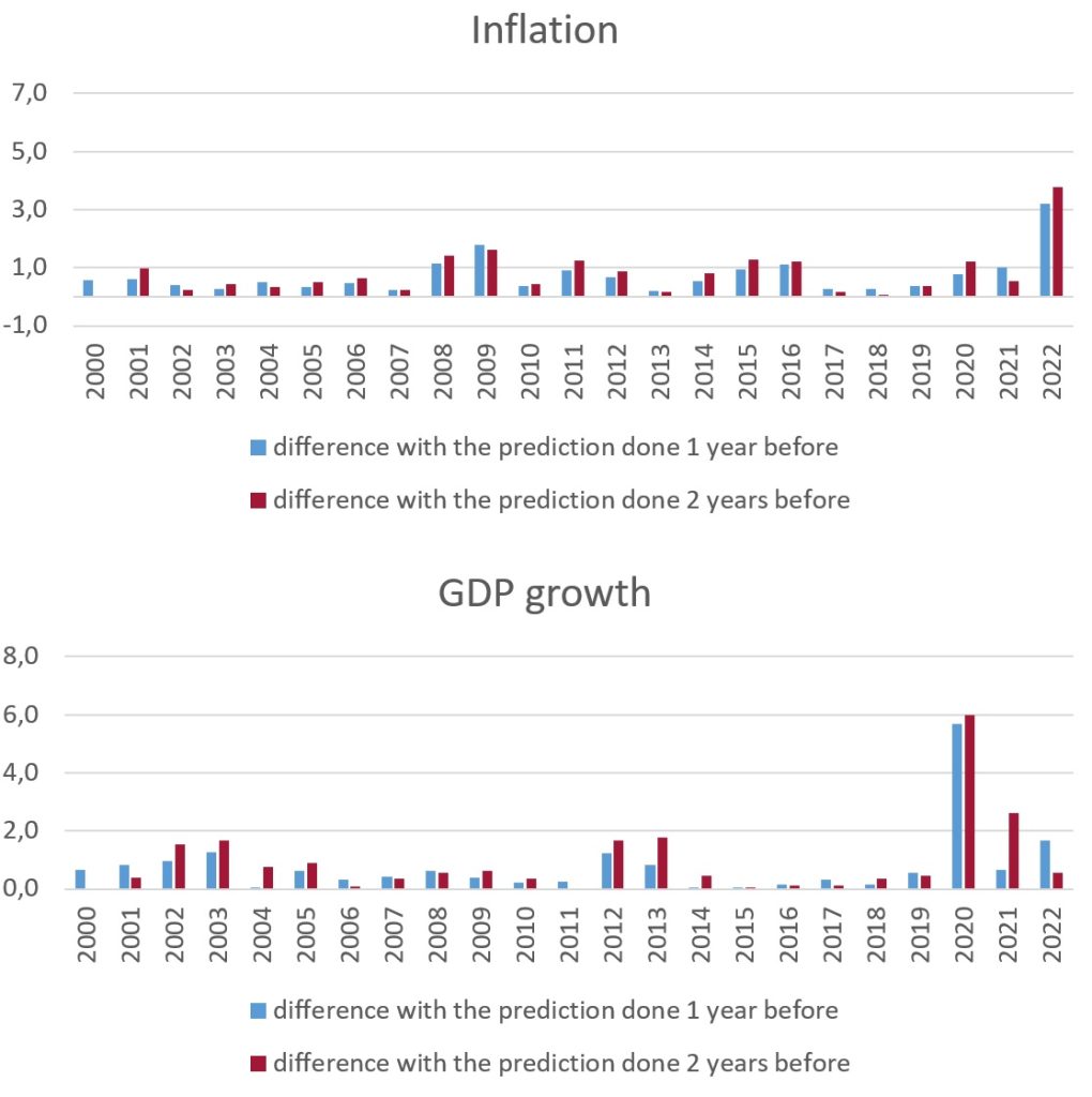
Source: Bruegel based on ECB. Note: The bars represent the changes over time of the yearly average inflation (Harmonised ICP, annual averages of quarterly forecasts) and GDP growth (Real GDP, annual averages of quarterly forecasts) forecasts expressed in absolute value. The dates correspond to the time at which the forecast is made, ie t+i in equation 1 in the Appendix.
Figure 1 shows the extraordinary uncertainty created first by COVID-19, in 2020 on growth, and then by the war in Ukraine, in 2022 on inflation: the corresponding changes in the forecasts of inflation and GDP growth are a large multiple of the average change since the introduction of the euro, and are higher than in any period since 2000. The Great Financial Crisis (GFC) is visible in the high uncertainty about inflation in 2008-2009.
To achieve a synthetic representation of our results, we averaged the changes in the ECB, IMF and SPF forecasts over the different time horizons available (3m, 1Y, 2Y)[1], as shown in Figure 2.
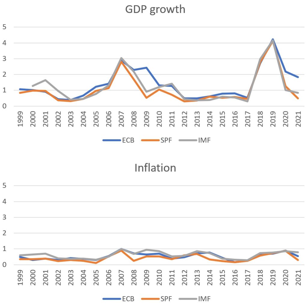
Figure 2: Changes in the ECB, IMF and SPF forecasts averaged over the different time horizons (inflation and GDP growth, percentage points difference)
Source: Bruegel based on ECB. Note: The lines represent the changes over time of the yearly average inflation (Harmonised ICP, annual averages of quarterly forecasts) and GDP growth (Real GDP, annual averages of quarterly forecasts) forecasts expressed in absolute value.
Figure 2 shows clearly that there have been two episodes of exceptional uncertainty during the life of the euro: the GFC of 2007-2008 and the COVID-19 crisis of 2019-2020. By far the greatest inflation uncertainty occurred, however, at the beginning of 2022, when the inflationary consequences of the war in Ukraine came on top of pre-existing inflationary trends. Also remarkable is that, for both inflation and GDP, uncertainty during the COVID-19 crisis has been, according to our metric, twice as intense as during the GFC. Equally interesting is that the changes in the GDP forecasts are, both during crises and in normal times, much greater than changes in inflation forecasts, indicating that shocks to GDP are more intense than shocks to inflation. This result is prima facie surprising, since the inflationary process does not have, per se, physical constraints like those on GDP growth. However, the broad success of the ECB in keeping, for much of the existence of the euro, inflation close to its target of 2 percent focused forecasters on a narrow range of options, so it is natural that changes in their forecasts were smaller than those relating to GDP. A final interesting remark is that the years preceding the Great Financial Crisis look very calm relative to what has happened since. The observation in Rostagno et al (2021) that the first eight years of the life of the euro were less affected by shocks than subsequent years is confirmed by our measure.
3 Forecasting errors by the three institutions
This section focuses on differences between forecasts and actual values, so-called forecasting errors. We calculated the forecasting error for the prediction for the same year, one year and two years ahead, and took the average of those values.
Figure 3: Yearly average over the different time horizons of forecasting errors (inflation and GDP growth, percentage points difference)
Source: Bruegel based on ECB Statistical Data Warehouse and World Economic Outlook (WEO). Note: The lines represent the forecasting errors of the yearly average inflation (Harmonised ICP, annual averages of quarterly forecasts) and GDP growth (Real GDP, annual averages of quarterly forecasts) forecasts expressed in absolute value.
Similarly to Figure 1 and 2, the financial crisis and the COVID-19 crisis are identified in Figure 3 as very uncertain periods. Uncertainty about the GDP growth rate is greater than uncertainty about inflation. When we look at GDP growth, we see that the COVID-19 crisis introduced more uncertainty than the financial crisis. We do not see yet the impact of Russia’s invasion of Ukraine on errors in predictions since we use annual data. However, in section 8, we show the most recent developments and the introduction of forecast scenarios.
We also observe that the ECB is the most reluctant of the three institutions to change its forecasts of GDP growth (Figure 2), and thus, its forecast errors were greatest on average (Figure 3). That observation led us to investigate differences in institutions forecasts.
4 Inter-institutional forecast differences
We assume that the difference between institutions in predictions for the same period increases when uncertainty is greater. Therefore, we constructed a time series showing the average difference between ECB forecasts and those of the IMF and SPF.
Figure 4: Yearly average of forecast differences between the ECB and the IMF/SPF (inflation and GDP growth, percentage points difference)

Source: Bruegel based on ECB Statistical Data Warehouse and World Economic Outlook (WEO). Note: The lines represent the changes over time of the yearly average inflation (Harmonised ICP, annual averages of quarterly forecasts) and GDP growth (Real GDP, annual averages of quarterly forecasts) forecasts expressed in absolute value.
Figure 4 confirms that the GFC and COVID-19 caused intense uncertainty, in particular over GDP growth. The figure also confirms that inflation is less affected by uncertainty than GDP growth.
5 Dispersion of forecasts of individual professional forecasters
The ECB SPF covers more than a hundred experts employed by financial and non-financial institutions, including economic research institutions (ECB, 2022b). Professional forecasters give their forecasts for several different horizons. For our analysis, we considered forecasts for the current calendar year, the next calendar year and the calendar year after that. Since the patterns of the different horizons are not significantly different, we only report the dispersion of forecasts for the 12-month horizon.
Figure 5: Dispersion of inflation and GDP growth forecasts among individual professional forecasters (inflation and GDP growth, percentage points difference)
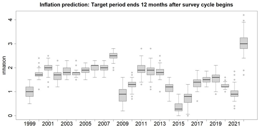
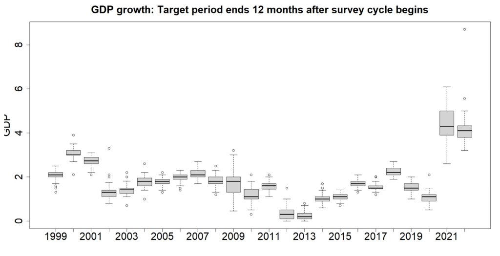
Source: Bruegel based on ECB Statistical Data Warehouse. Note: Each grey box represents the first quartile up to the third quartile, with a black line inside representing the median. The minimum and maximum are shown by black lines outside each box, connected to the box by dotted lines. Dots represent outliers. Inflation is defined as Harmonised ICP (annual averages of quarterly forecasts) and GDP growth as a real GDP (annual averages of quarterly forecasts).
The data shows that the dispersion of forecasts for GDP growth in 2021, and for inflation in 2022, are the largest since the launch of the euro. Also, for professional forecasters, GDP growth is more prone to uncertainty than inflation. Different time horizons, beyond the shortest-term inflation prediction, confirm that the variation is greatest for GDP growth in 2021 and inflation in 2022.
6 An overall reading of the evidence about uncertainty
Our measure of uncertainty indicates the following four stylised facts:
- Uncertainty was by a significant degree greater during the GFC and the COVID-19-Ukraine crisis than on average since the creation of the euro, but:
- In the latter crisis, uncertainty has been even greater than in the former, and thus the current crisis is causing the greatest uncertainty since the introduction of the euro;
- Uncertainty over the real growth process is more intense than that for inflation;
- Forecasters may be caught out by crises because they are looking at the wrong information.
7 Which component prevails in the stagflationary shock from the war in Ukraine?
While it is clear that the war in Ukraine has imparted a stagflationary shock to the European Union economy, it is interesting to identify which of the two components – the stag- or the –flationary shock – prevails.
To do this, following the same logic as in sections 3 and 4, the relative intensity of the stag- to the –flationary component of the shock was derived by comparing the change of the inflation forecast (inflation component) with the change in the growth forecast (the growth component). For comparison purposes, the same exercise was then done using data from the Great Financial Crisis period. Figure 6 details the results.
Figure 6: Deviations between the three institutions’ forecasts in 2021 for 2022 (Ukrainian war) and 2008 for 2009 (GFC), percentage points difference
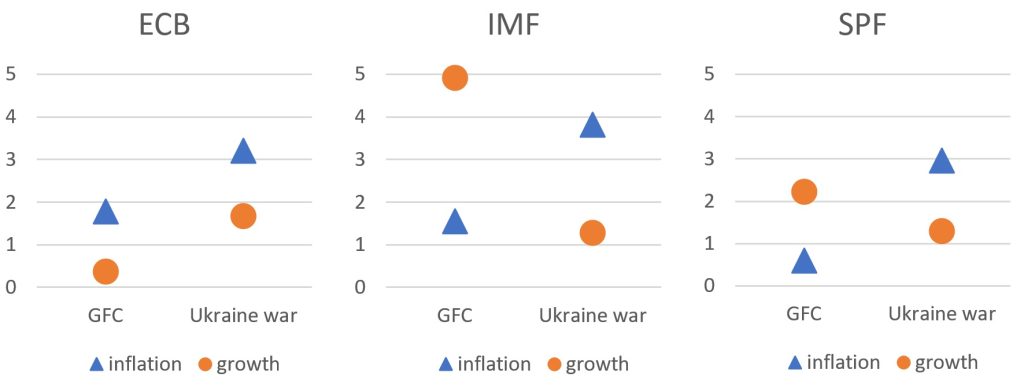
Source: Bruegel based on ECB Statistical Data Warehouse and World Economic Outlook (WEO). Note: The difference is expressed in absolute value. Inflation is defined as Harmonised ICP (annual averages of quarterly forecasts) and GDP growth as a real GDP (annual averages of quarterly forecasts).
According to each of the three institutions, the inflationary component of the shock coinciding with the Ukraine war has been much worse (as the inflation forecast was revised upwards by 3 percent or more) than at the time of the GFC (less than 2 percent). However, according to the IMF and the SPF, the growth component of the shock during the GFC outstripped the inflation component (for the ECB the result was different). Overall, we can characterise the Ukraine crisis as an inflation event, and the GFC as a growth event. One other result common to the three institutions is that in the Ukraine crisis, the inflationary component of the shock is about twice as large, in absolute terms, as the growth component.
The characterisation of the Ukraine war shock as much more inflationary than recessionary allows us to qualify the traditional conclusion according to which monetary policy should look through stagflationary shocks and neither fight inflation, aggravating the recession, nor fight the recession, worsening the inflationary situation. Indeed, the much heavier inflationary component of the shock provides justification for prioritising the fight against inflation in current circumstances.
8 Which macroeconomic pattern is expected to prevail in the medium term?
Table 1 updates the table in Grzegorczyk et al (2021), which showed a convergence of forecasts towards a return to the pre-COVID-19 pattern. Table 1 seems to confirm this, showing an expected return to normal both for inflation and growth between 2023 and 2024.
This is somewhat surprising considering that the deglobalisation, or reshoring, phenomenon, which COVID-19 and then the Ukraine war has caused, is often assumed to reduce productivity, and hence growth, on a persistent basis. The forecasts for 2023 and 2024 in the table conform instead with a pattern according to which the economy is hit by a shock that gradually dissipates and returns to the equilibrium prevailing before the crisis. This is possible but is contrary to the fear that the two crises will leave persistent scars on the economy.
Table 1: Medium term scenarios, growth and inflation for the euro area
| GDP growth | Inflation (HICP) | |||
| Past observation: Q3 2021 | Current observation: Q1 2022 | Past observation: Q3 2021 | Current observation: Q1 2022 | |
| IMF | 2021: 5.0% 2022: 4.4% 2023: 2.0% | 2022: 2.8% 2023: 2.3% 2024: 1.8% | 2021: 2.2% 2022: 1.7% 2023: 1.4% | 2022: 5.3% 2023: 2.3% 2024: 1.8% |
| ECB | 2021: 5.0% 2022: 4.6% 2023: 2.1% | 2022: 3.7% 2023: 2.8% 2024: 1.6% | 2021: 2.2% 2022: 1.7% 2023: 1.5% | 2022: 5.1% 2023: 2.1% 2024: 1.9% |
| OECD | 2021: 5.3% 2022: 4.6% | 2022: 4.3% 2023: 2.5% | 2021: 2.1% 2022: 1.9% | 2022: 2.7% 2023: 1.8% |
| Goldman Sachs | 2021: 4.9% 2022: 4.3% 2023: 2.0% 2024: 1.3% | 2022: 2.5% 2023: 1.9% 2024: 1.9% | 2021: 2.3% 2022: 2.0% 2023: 1.3% 2024: 1.4% | 2022: 7.3% 2023: 3.5% 2024: 1.9% |
| CITI | 2021: 5.2% 2022: 4.7% | 2022: 2.4% 2023: 2.7% | 2021: 2.3% 2022: 2.0% | 2022: 7.2% 2023: 2.8% |
Source: Bruegel based on Bloomberg.
The forecasts in Table 1, however, do not illustrate sufficiently the conditions on which the euro-area economy is forecast to converge. What is missing is the fact that, confronted with exceptional uncertainty, forecasters have moved to a methodology in which, instead of a central forecast, different scenarios are produced, without specifying their probability.
Although institutions started discussing different scenarios with downside risks in 2020, the ECB introduced a systematic release of scenarios only in March 2020. Figure 7 reports the ECB’s inflation and growth projections published in the third quarter of 2021, and those published in the first quarter of 2022. These forecasts show, in line with Figure 1, above, a significant decrease in GDP growth and an even larger increase for inflation, in all scenarios in 2022. However, the Ukraine war has not significantly changed the growth projections for 2023 and 2024, even in the severe scenario. The ECB explained that even if the Ukrainian war has a negative impact on euro-area growth, the Next Generation EU programme should boost investment. In addition, all scenarios assume that there will be a resolution of the conflict over time. Inflation is forecast to take one more year, until 2024, to move towards 2 percent, but it is assumed to do so under all three scenarios (ECB, 2022a).
Thus, also looking at the different scenarios, forecasts still gravitate towards the pattern prevailing before the COVID-19-Ukraine crisis, with both inflation and growth at around 2 percent.
Figure 7: ECB different scenarios (inflation and GDP growth, percentage points difference)
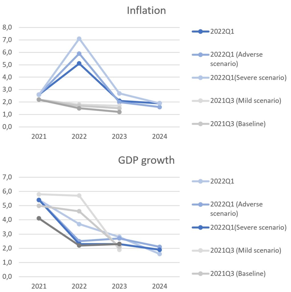
Source: Bruegel based on ECB staff macroeconomic projections for the euro area.
9 Conclusions
We conclude from our analysis that macroeconomic uncertainty was, by a significant degree, greater during the GFC and the COVID-19-Ukraine crisis than the average since the creation of the euro. In addition, in the latter crisis, uncertainty has been even greater than in the former. The current crisis is thus causing the most intense uncertainty in the lifetime of the euro. Moreover, the uncertainty affecting the real growth process is more intense than that affecting the inflation process.
Our analysis supports the widespread belief that the Ukraine shock is more inflationary than recessionary, justifying monetary tightening.
Surprisingly, our results also show that, notwithstanding the intensity of the uncertainty during the COVID-19-Ukraine crisis, the euro-area economy is assumed to converge around 2024 back towards the pattern prevailing before the crisis, with both inflation and growth at around 2 percent.
References:
Bank of England (2013) ‘Macroeconomic uncertainty: what is it, how can we measure it and why does it matter?’ Quarterly Bulletin 2013 Q2, available at https://www.bankofengland.co.uk/-/media/boe/files/quarterly-bulletin/2013/macroeconomic-uncertainty-what-is-it-how-can-we-measure-it-and-why-does-it-matter.pdf
Ben-David, I., E. Fermand, C.M. Kuhnen and G. Li (2018) ‘Expectations Uncertainty and Household Economic Behavior’, Working Paper 25336, National Bureau of Economic Research, available at https://www.nber.org/papers/w25336
Bennett N. and G.J. Lemoine (2014) ‘What VUCA Really Means for You’, Harvard Business Review, January-February, available at https://hbr.org/2014/01/what-vuca-really-means-for-you
Bloom N. (2009) ‘The impact of uncertainty shocks’, Econometrica 77(3): 623–685, available at https://pages.stern.nyu.edu/~dbackus/GE_asset_pricing/Bloom%20uncer%20shocks%20Ec%2009.pdf
Coibion O., D. Georgarakos, Y. Gorodnichenko, K. Kenny and M. Weber (2021) ‘The Effect of Macroeconomic Uncertainty on Household Spending’, IZA Discussion Paper No. 14213, available at https://ftp.iza.org/dp14213.pdf
ECB (2022a) ECB staff macroeconomic projections for the euro area, March, European Central Bank, available at https://www.ecb.europa.eu/pub/projections/html/ecb.projections202203_ecbstaff~44f998dfd7.en.html
ECB (2022b) Background on the survey of professional forecasters, European Central Bank, available at https://www.ecb.europa.eu/stats/ecb_surveys/survey_of_professional_forecasters/html/about_the_survey.en.html
Gieseck A. and S. Rujin (2020) ‘The impact of the recent spike in uncertainty on economic activity in the euro area’, ECB Economic Bulletin 6/2020, available at https://www.ecb.europa.eu/pub/economic-bulletin/focus/2020/html/ecb.ebbox202006_04~e36366efeb.en.html
Gilchrist S., J.W. Sim and E. Zakrajsek (2014) ‘Uncertainty, Financial Frictions, and Investment Dynamics’, Working Paper 20038, National Bureau of Economic Research, available at https://www.nber.org/papers/w20038
Grzegorczyk, M., F. Papadia and P. Weil (2021) ‘Is the risk of stagflation real?’ Bruegel Blog, 2 November, available at https://www.bruegel.org/2021/11/is-the-risk-of-stagflation-real/
McMahon, M. (2020) ‘Why is uncertainty so damaging for the economy?’ Economics Observatory, 29 May, available at https://www.economicsobservatory.com/why-uncertainty-so-damaging-economy
Rostagno M., C. Altavilla, G. Carboni, W. Lemke, R. Motto, A. Saint Guilhem and J. Yiangou (2021) Monetary Policy in Times of Crisis, Oxford University Press
Sgaravatti, G., S. Tagliapietra and G. Zachmann (2021) ‘National policies to shield consumers from rising energy prices’, Bruegel Datasets, first published 4 November, available at https://www.bruegel.org/publications/datasets/national-policies-to-shield-consumers-from-rising-energy-prices/
Theophilopoulou A. (2021) ‘The impact of macroeconomic uncertainty on inequality: An empirical study for the United Kingdom’, Journal of Money, Credit and Banking 54(4): 859-884, available at https://doi.org/10.1111/jmcb.12852.
Appendix: A measure of macroeconomic uncertainty
The specific definition of macroeconomic uncertainty we measure starts from the following equation:
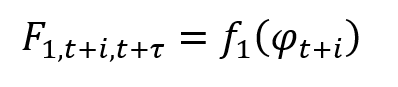
For i = 0,… ,3 and 𝜏=1,…,3
Where:
is the forecast of institution 1 made at time t+i for period 𝑡+𝜏 and 𝜏 is the forecast horizon.
Changes in F1 are transformations of changes in ϕ, ie seeing how over time institution 1 changes its forecast for period we measure changes in the macroeconomic information set determining the forecast.
Greater changes lead to more uncertainty.
Of course, when a forecast is made at the same time as the actual value of the macro variable is revealed, ie F1,t+i,𝑡+𝜏 , then the forecast revision is the same as the forecasting error. Indeed, in the text we use this latter denomination for the forecasting change in this specific case.
Analogously, assuming that macroeconomic uncertainty leads institution 1 to a different forecast from that of institution 2, because

the different forecasts from different institutions can also be taken as an indication of uncertainty.
The formula for indicator 1 in the main text is:

For i = 0,… ,3
ie the forecast of institution 1 for period 𝑡+𝜏 made at time 𝑡+i minus the forecast of institution 1 for the same period 𝑡+𝜏 made at time 𝑡+i+1
The formula for indicator 2 is:

ie the forecasting error between the forecast made at time t and the forecast at time 𝑡+𝜏 that is the same as the realisation of the relevant variable.
The formula for indicator 3 is:
where dt is the forecast deviation between institution 1 and institution 2 made at time t for time 𝑡+𝜏
The precise time indexing of indicators 1 and 2 in the main text is explained in the following table:
| 𝜏 | 0 | 1 | 2 | 3 |
| 1 | t,t+1 | t+1,t+1 | – | – |
| 2 | t,t+2 | t+1,t+2 | t+2,t+2 | – |
| 3 | t,t+3 | t+1,t+3 | t+2,t+3 | t+3,t+3 |
| Average | (t,t+1+ t,t+2)/2 | (t+1,t+1+t+1,t+2)/2 | (t+2,t+2) | t+3,t+3 |
Uncertainty indicators 1 and 2 in the main text are given by the difference between a cell and the adjacent cell on the right. The bottom row defines the averages used in Figures 2, 3 and 4.
[1] We do not consider the 3-year horizon in the average since it is not available for all years in the sample.
