Does money growth tell us anything about inflation?
Together with Cadamuro Leonardo
Economists and central bankers no longer consider monetary aggregates relevant for inflation forecasts. We explain this neglect by advancing and testing the hypothesis that monetary aggregates are only relevant for inflation in unsettled monetary and inflationary conditions. When inflation is basically stable around the central bank target (1.9 percent), as it has been in most of the last two decades, there is no apparent relationship between monetary aggregates and inflation. This is not surprising: there is not much to be explained about a constant. However, attention should be paid to a possible sequence of negative events: if inflation would start to be volatile and money growth remains high, efforts to control inflation could be undermined.
1 The salience of money for the European Central Bank, economists and the general public.
In the view of economists, money seems to have lost its relevance for forecasting, let alone explaining, inflation. In the European Central Bank’s 2021 monetary policy strategy review (see ECB, 2021), there is indeed a reference to “a weakening of the empirical link between monetary aggregates and inflation”. And the economic and the monetary pillars of the ECB strategy have disappeared, transformed into an “integrated analytical framework that brings together two analyses: the economic analysis and the monetary and financial analysis”. Only as a sort of afterthought is it said that: “The integrated analytical framework will continue to consider the information from monetary and credit aggregates”1.
However, a Google search for the word ‘money’ and its cousins (monetary aggregates, M1, M2, M3) for the euro area and the United States is not consistent with this irrelevance hypothesis. The frequency of the word ‘money’, in particular in its narrower definition of M1, has increased quite abruptly since the end of 2019 (Figure 1). In Figure 1 and subsequent figures, the shaded area starting in March 2020 highlights the ‘pandemic observations’.
Figure 1: Frequency of Google searches for ‘money’ and related terms, January 2004 to September
2021

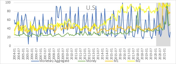
Source: Bruegel. Note: The variable on the vertical axis is the frequency for each month of searches for the word ‘money’ indicates the minimum value and 100 the maximum value.
The disappearance of money from economists’ description of inflation but not from the public narrative, as arguably represented by Google searches, is not surprising. While De Grauwe and Polan (2005) convincingly showed that the quantity theory of money is not a universally applicable model for understanding inflation, the theory remains popular 2. This is encapsulated by the idea of ‘too much money chasing too few goods’. In symbols, it is expressed as:
Eq. 1 MT=PQ
Where M is a monetary aggregate, ܶT is the velocity of money, ܲP is the price level and ܳQ is real income. And the accounting identity is transformed into an economic statement by assuming ܶT is constant (or just independent of M), while ܳQ is exogenous and thus does not respond to changes in M, assumed in turn to be a policy variable. With these assumptions, M determines ܲP
The European Central Bank in 1999 started with a somewhat more sophisticated version of the quantity theory of money as one of the two pillars of its strategy. Fischer et al (2009) described it as follows: “At the beginning of Stage III, the assessment of monetary developments was focused on an analysis of the deviations of M3 growth from the ECB’s reference value of 4.5%”. The 4.5 percent reference value was, in turn, derived by adding up, and trimming, a target inflation rate of 2 percent, real growth between 2 percent and 2.5 percent and a decline in the velocity of M3 by 0.5 percent to 1.0 percent per year. Establishing a reference value for M3 was justified by the fact that, “In the past, the demand for euro area broad money has been stable over the long run. Broad aggregates have been leading indicators of developments in the price level”3. The reference value for M3 clearly derived from the Bundesbank experience but was also consistent with the approaches of the Banque de France and Banca d’Italia. The word ‘credit’ was not mentioned in the initial monetary policy strategy, only being referred to, with some disdain, as “counterparts” to monetary aggregates.
The disappointment caused by the instability in the demand for money, which made the “reference value” impractical as a guide for monetary policy, gradually led to a more subtle use of the ‘monetary pillar’. This was already evident in 2006, at a major conference organised by the ECB, arguably to defend the role of money in monetary policy. At that conference the main paper, prepared by Fischer et al (subsequently Fischer et al, 2009), clearly stated that: “there is no reliable estimated money demand equation which covers the entire sample period”, thus recognising that a straightforward use of money aggregates for monetary policy was not possible. The paper proposed, however, “a holistic assessment of the monetary data” to better understand economic developments and forecast inflation. At the same conference, then ECB chair, Jean-Claude Trichet (2008), argued that looking at broad monetary and credit developments helped the ECB: first, to assure “continuity with the most credible central banks joining the Eurosystem”; second, to identify financial imbalances; and third, to qualify, in some special circumstances, the information from the so-called economic analysis. Also, former members of the ECB’s board, Otmar Issing and Jurgen Stark, supporters of the importance of money, at the 2006 conference substantially diluted the idea that monetary policy should be guided by deviations of M3 from the reference value, adopting a more generic statement that money deserves a prominent, but variable, role in monetary policy (Issing, 2008; Stark, 2008).
Gradually, the second pillar of the ECB monetary policy strategy moved from being the broader of the two (Issing, 2008) to become a ‘pillarette’, a complement to the most important economic analysis, and, within this ‘pillarette’, credit developments got more attention than monetary developments.
2 One view about the link between money and inflation
The view of one of the authors of this paper about the relationship between money and inflation can be summarised in two anecdotes. The first concerns a seminar at Banca d’Italia in the 1970s, when the author asked economics Nobel Prize winner Paul Samuelson whether he agreed with the weak form of monetarism according to which extreme things are likely to happen to prices when extreme things happen to money. If memory serves well, Samuelson conceded that much, while remaining very far from endorsing any kind of Friedmanian monetarism. Second, the author advanced at the 2006 ECB conference “the hypothesis that the importance of money in monetary policy is not constant and depends on the level and uncertainty of inflation . . . Attributing much weight to monetary aggregates helps moving from high and unstable inflation to low and stable inflation but when the new level of lower inflation has been achieved money would turn from being very important to being just relevant”. Michael D. Bordo (2008), also attending the conference, expressed the same view.
This view can be summarised in the statement that money matters for inflation in unstable conditions characterised by high rates of growth of money and/or inflation. De Grauwe and Polan (2005) showed empirically that this is indeed the case: the strong link between inflation and money only emerges in high or hyper-inflation countries, when inflation is lower than 10 percent, the link is weak or absent. On this basis, already in 2005, they advised the ECB against taking money growth as a useful signal of inflationary conditions.
3 A testable version of the hypothesis that money matters in unsettled conditions.
Based on the considerations discussed so far, we identify a general, but empirically testable hypothesis: only when monetary/inflationary developments are unsettled does money provide information for inflation forecasting. We start by testing this hypothesis against recent developments. Figure 2 reports the growth rates of M1, M2, M3 and inflation in the euro area, where, of course, data from before 1999 is a weighted average of the countries that would adopt the euro in that year.
Figure 2: Rates of growth of M1, M2, M3 and inflation, euro area, January 1971 to June 2021
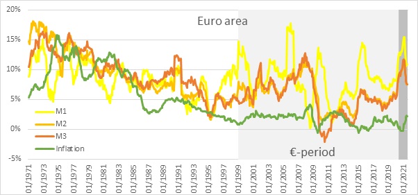
Source: Bruegel based on European Central Bank – Eurosystem, Money, credit, and banking dataset, monetary aggregates.
Figure 2 shows:
- A trend of decreasing inflation since the middle 1970s and relative stability since the
introduction of the euro; - Overall greater volatility for monetary aggregates, particularly for M1, than inflation;
- Higher rates of growth for monetary aggregates in the 1970s and 1980s than in the following
decades; - A new spike in the growth of money aggregates in ‘pandemic months’, starting in March 2020.
Figure 3 reports similar variables for the United States.
Figure 3: Rates of growth of M2 and inflation, United States, January 1971 to June 2021

Source: Bruegel based on Federal Reserve website, Data Download Program. Note: The M3 series was discontinued by the FED in 2006, as it was considered no longer relevant for monetary policy, while the M1 series is affected by a definitional change carried out in May 2020 and is thus excluded.
In Figure 3:
- The most visible phenomenon is the spike in M2 in the US during pandemic months, with a rate of growth exceeding 25 percent, by far the highest in the last half century;
- In comparison with the euro area, there is overall less volatility in money growth;
- Inflation has been fairly stable since the middle 1980s, when the Great Moderation started;
- There is no obvious correlation between monetary aggregates and inflation.
Based on the evidence shown in Figures 2 and 3, inflationary developments have not been unsettled in either the euro area or the US, while monetary developments have only shown a spike recently, especially in the US.
To better gauge monetary developments during pandemic months, we present in the two following figures the frequency distribution of the growth of the inverse of velocity of money (i.e. nominal money divided by nominal GDP, 1/T in the symbols of Eq. 1), in the US and in the euro area over the last half century. The blue bars denote 1 and 2 standard deviations of growth rates away from the average (green bar), while the pandemic observations are in a darker colour and circled. The analysis is limitedto to M1 and M3 for thew euro area, since the correlation index between M2 and M3 is 0.93, and to M2 in the US, fot the reasons explained in the note to FIgure 3.
Figure 4: Frequency distribution of rates of growth of the inverse of velocity of M1 and M3, euro area, January 1971 to June 2021
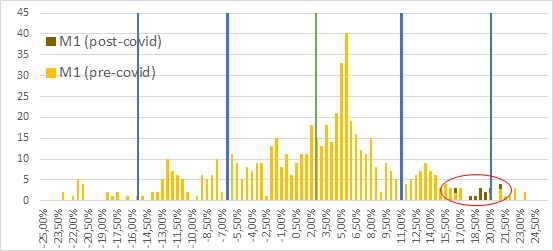

Source: Bruegel
The pandemic observations for the inverse of money velocity are pushed to the right by the fall in GDP resulting from the pandemic: their rates of growth are, in the European Union, 1 or 2 standard deviations above the mean for M1 and M3.
Figure 5: Frequency distribution of rates of growth of the inverse of velocity of M2, United States, January 1971 to June 2021

Source: Bruegel
In the case of the United States, the pandemic observations of the growth of the inverse of the velocity of money are exceptionally high as they are well beyond the 2 standard deviation limit.
In conclusion, while the peak of monetary growth has been extreme in the US in the pandemic period, it is only the behaviour of M1 in the euro area that can be qualified as unsusal. However, in both the euro area and the US, the volatility during the pandemic months has not been sustained enough to define monetary conditions as unsettled: so far, this looks more like an episode than a new pattern. In conclusion, neither inflationary not monetary conditions can currently be defined as unsettled. According to our hypothesis, we should not find strong indicators for inflation in monetary developments. This is indeed what we document in the next section.
4 Money supply developments do not help in forecasting inflation in settled conditions
To test the hypothesis that, in settled conditions, money does not provide information on price developments, either upwards or downwards, we conducted the following experiment. First, an equation, as in Fischer et al (2009), was estimated with all the observations between 1970 and 1998 for the euro area and the US:
Eq. 2 πt+h=a+b1πt-1+…+bpπt-p+c1xt-1+…+cpxt-p+εt+h
Where:
π represents inflation
x represents money growth
and the data is quarterly to avoid the spurious autocorrelation of residuals caused by overlapping observations. The estimates of this regression were then used to forecast inflation one quarter ahead, starting in the first quarter of 1999, updating the regression estimate quarter by quarter. In a way, it is as if, at the beginning of the life of the euro, an economist tried to forecast inflation, in the euro area as well as in the US, on a rolling basis using lagged inflation and money growth. In the appendix, we report results for the same exercise run with only observations of M1 and M3 for the euro area and of M2 for the US that exceed 1 standard deviation, upward and downward, to check whether during this period higher rates of growth of money carried more information for subsequent rates of inflation.
Overall, this is not the case: a burst of high money growth does not make money more relevant in forecasting inflation.
Table 1: Measuring the performance of different inflation forecasting models, euro area, out of sample forecasts, January 1999 to June 2021
| Forecasting Model | MSFE |
| Auto Regression | 0.00001 |
| Random walk | 0.00354 |
| Fixed 1.9% | 0.00010 |
| Adding M3 | 0.00184 |
Source: Bruegel.
Table 1 shows the results for the euro area, comparing the mean square forecasting error (MSFE) of four forecasting models. To check whether money growth improves the inflation forecast, the MSFE calculated from the regressions with money, as in Eq. 2, was compared to three naïve forecasts: an autoregressive moving average, a random walk and a fixed forecast corresponding to the ECB’s inflation objective (1.9 percent). When Fischer et al (2009) estimated their forecasts, the random-walk forecast beat by a good margin the forecast based on money, while the best non-composite forecast resulted from trusting that the ECB would have achieved its objective to stabilise inflation around 1.9 percent.
We found, with our much longer time series, that, in the period since the introduction of the euro:
- Like Fischer et al (2009) a pretty good forecast would have been achieved assuming that the ECB would have run the show well and kept inflation close to 1.9 percent;
- Contrary to Fischer et al (2009) we found that a bivariate forecast, with M3 added to lags of inflation, would have reduced the forecast error relative to a random walk forecast, but the MSFE is still, in this case, much higher than the constant and the autoregressive forecast, the latter having the lowest MSFE.
Table 2: Measuring the performance of different inflation forecasting models, United States, out of sample forecasts, January 1999 to June 2021
| Forecasting Model | MSFE |
| Auto Regression | 0.00002 |
| Random walk | 0.00176 |
| Fixed 1.9% | 0.00015 |
| Adding M2 | 0.00096 |
Source: Bruegel.
The results for the US are like those for the euro area:
- The best forecast for the 1999-2021 period is the autoregressive moving average, but the forecast deriving from the assumption that the Fed would keep inflation close to its target of 2 percent is quite close;
- Forecasting inflation with the help of money does improve with respect to a random walk forecast but not with respect to an autoregressive moving average and the fixed 1.9 percent assumption.
On reflection, it is not surprising that good forecasts come from assuming a constant 1.9 percent inflation rate: Figures 2 and 3 show that actual inflation stayed very close to that level and the best forecast of a constant is, trivially, a constant. There is an analogy here with the relationship between fuel consumption and speed in a car with cruise control: at the end of a trip during which the car always ran at a constant speed, there would be no point looking for a relationship between fuel consumption and speed, even if we know that it exists, because the cruise control system has kept the speed constant. And fuel consumption, the counterpart of money in our set up, would be more volatile (because of wind, going up and down hills) than speed, the counterparty of inflation in the analogy. As seen in Figures 2 and 3, this is just what happens.
Overall, we do not find that money helps to forecast inflation over the 1999-2021 period either in the euro area or the US: the naïve, but institutionally based, assumption that both the Fed and the ECB stayed close to their objectives produces quite good forecasts. This also means that the approach of looking at inflation prospects without considering monetary aggregates is not contradicted by our results, at least in today’s circumstances.
Still the results so far do not necessarily contradict the hypothesis, formulated above, about money being relevant in unsettled conditions: money may not help improve forecasts just because, between 1999 and 2021 for the euro area and the US, inflationary/monetary developments have not been variable enough. Central bank cruise control was at work.
This conclusion is reinforced considering, as shown by Anderson et al (2021), that there was at the beginning of the pandemic an exceptional increase in bank lending in the four largest euro-area countries, and arguably across the region, because of the very large guarantee programmes established by governments to prevent businesses from failing because of illiquidity. The liquidity obtained through the abundant bank lending was, to a great extent, deposited with banks, thus inflating monetary aggregates. A similar phenomenon occurred in the US (see for example Cheng et al, 2021), following the role of the Fed in promoting an extraordinary bank lending programme, the proceeds from which were partially deposited with banks. In addition, a large share of the special liquidity support from the federal government went into bank accounts, thus swelling money supply. It is thus possible that, as the economy recovers from the pandemic, both bank lending and bank deposits will return to a normal path, in which case the increase in monetary aggregates documented above would be just a temporary phenomenon, without permanent inflation effects. The latest, more moderate, observations of money growth at time of writing support this interpretation.
5 Monetary developments help to forecast inflation in unsettled conditions
To further test the hypothesis that monetary developments only help in forecasting inflation in unsettled circumstances, we can look for periods characterised by more inflation and money growth variability than in the recent decades – the 1975-1985 period for the US and the pre-euro period for the euro area.
To do this, we carried out the same exercise as above, but we forecast the 1975-1998 period, ie the pre-euro period, for the euro area and the 1975-1985 period for the US, ie the pre-Great Moderation period. The first regression in the forecasting exercise was estimated using the first five years of observations.
Table 3: Measuring the performance of different inflation forecasting models, euro area, out of sample forecasts, January 1975 to January 1998
| Forecasting Model | MSFE |
| Auto Regression | 0.00602 |
| Random walk | 0.00308 |
| Fixed 1.9% | 0.00386 |
| Adding M3 | 0.00167 |
Source: Bruegel.
The results for the euro area show that:
- Of course, now the constant 1.9 percent forecast performs poorly with a high MSFE;
- Also, the autoregressive moving average and the random-walk forecasts show high MSFE;
- The forecast using money is more precise than any other forecast.
Table 4: Measuring the performance of different inflation forecasting models, United States out of sample forecasts, 1975-1985
| Forecasting Model | MSFE |
| Auto Regression | 0.00657 |
| Random walk | 0.00180 |
| Fixed 1.9% | 0.00412 |
| Adding M2 | 0.00171 |
Source: Bruegel.
The results for the US show that:
- The best performance is achieved by using M2;
- The three naive forecasts (fixed 1.9 percent, random walk and autoregressive moving average) produce larger MSFE.
In conclusion, unlike in the time periods in which inflation was fairly stable (1999-2021 for the euro area and 2000-2021 for the US), money helps forecasting inflation. We thus get a first piece of evidencee that money matters when the monetary/inflationary situation is unsettled. To further check whether the importance of money to forecast inflation depends on the volatility of inflationary/monetary conditions, we carried out a similar exercise for a country undergoing more severe monetary instability: Italy in the 1970s and 1980s.
Figure 6: Rates of growth of M2 and inflation in Italy in from 1957 to 1998.

Source: Bruegel based on M2 series published by Banca d’Italia and CPI published by Istat.
Figure 6 shows that M2 and inflation were very variable, with a peak of 25%-30% growth in the middle 1970s as well as a broad association between the two variables: a regression with the lagged valued of inflation and M2 explains inflation, denoting a strong autoregressive pattern. The out-of-sample forecasts confirm that money help in forecasting inflation in the unsettled 1970-1989 period in Italy, since the MSFE of the forecast using M2 is the lowest of the four models.
Table 5: Measuring the performance of different inflation forecasting models, Italy, out-of-sample forecasts, 1970-1989.
| Forecasting Model | MSFE |
| Auto Regression | 0.05743 |
| Random walk | 0.07554 |
| Fixed 1.9% | 0.05951 |
| Adding M2 | 0.04333 |
Source: Bruegel.
6 Conclusions
One conclusion from the evidence we have assembled is that money does not really help in forecasting inflation when inflation is close to stable. Indeed, if inflation remains close to the central bank objective, namely 2 percent, money has no forecasting power with respect to future inflation. However, when inflation is volatile, as in the pre-euro period in the euro area and before the Great Moderation in the US, money does help in forecasting inflation. This result is confirmed by looking at a country with a more severe problems of monetary instability, such as Italy in the 1970s and 1980s.
Overall, while, in contrast to the quantity theory of money, there is no constant relationship between money and inflation, in unsettled monetary and inflation conditions monetary developments do provide information relevant to inflation. However, it is not the sporadic extreme observations that matter, but a sustained pattern of high volatility. Our results, analogous to those of De Grauwe and Polan (2005), are more consistent with an economic-history approach, which aims to explain economic phenomena by taking path dependency into account, rather than by attempting to find time-invariant, universal economic relationships.
Currently, notwithstanding the recent increase, no pattern of inflation variability prevails, hence the acceleration of money provides no evident sign of coming inflation. Our results do not contradict the prevailing view that the recent increase in inflation, to 5.4 percent in the US and to 4.1 percent in the euro area, is temporary. Nor do they confirm this view, however.
Attention should be paid to a possible sequence of negative events: if inflation would start to be volatile and money growth remains high, efforts to control inflation could be undermined.
References:
Anderson, J., F. Papadia and N. Véron (2021) ‘COVID-19 credit-support programmes in Europe’s five largest economies’, Working Paper 03/2021, Bruegel, available at https://www.bruegel.org/2021/02/covid-19-credit-support-programmes-in-europes-five-largesteconomies/
Bordo, M.D. (2008) ‘Comment’ on ‘Pillars of globalisation: a history of monetary policy targets, 1797- 1997’, in A. Beyer and L. Reichlin (eds) The Role of Money – Money and Monetary Policy in The TwentyFirst Century, Fourth ECB Central Banking Conference, 9-10 November 2006, European Central Bank De Grauwe, P. and M. Polan (2005) ‘Is Inflation Always and everywhere a Monetary Phenomenon?’ Scandinavian Journal of Economics 107 (2): 239-259
ECB (1999) ‘The Stability-Oriented Monetary Policy Strategy of the Eurosystem’, Economic Bulletin,
January 1999, European Central Bank ECB (2021) An overview of the ECB’s monetary policy strategy, July, European Central Bank, available at https://www.ecb.europa.eu/home/search/review/pdf/ecb.strategyreview_monpol_strategy_overview.en
.pdf
Fischer, B., M. Lenza, H. Pill and L. Reichlin (2009) ‘Money and monetary policy: the ECB experience 1999-2006’, Journal of International Money and Finance, 28: 1138-1164
Issing O. (2008) ‘The ECB’s monetary policy strategy: why did we choose a two-pillar approach?’ in A. Beyer and L. Reichlin (eds) The Role of Money – Money and Monetary Policy in The Twenty-First Century, Fourth ECB Central Banking Conference 9-10 November 2006, European Central Bank
Stark J. (2008) ‘The role of the money’, in A. Beyer and L. Reichlin (eds) The Role of Money – Money and Monetary Policy in The Twenty-First Century, Fourth ECB Central Banking Conference 9-10 November 2006, European Central Bank
Trichet J.C. (2008) ‘Panel Discussion’, in A. Beyer and L. Reichlin (eds) The Role of Money – Money and Monetary Policy in The Twenty-First Century, Fourth ECB Central Banking Conference 9-10 November 2006, European Central Bank
- In the same line of thinking, Bruegel director Guntram Wolff in mid-2021 reached the reassuring conclusion that the “euroarea inflation forecasts do not show any sustained rise in inflation,” without once mentioning the word ‘money’ or similar. See Guntram Wolff, ‘Inflation!? Germany, the euro area and the European Central Bank’, Bruegel Blog, 9 June 2021, available at https://www.bruegel.org/2021/06/inflation-germany-the-euro-area-and-the- European-central-bank/. [↩]
- See Marek Dabrowski, ‘Monetary arithmetic and inflation risk’, Bruegel Blog, 28 September 2021, available at https://www.bruegel.org/2021/09/monetary-arithmetic-and-inflation-risk/. [↩]
- The monetary pillar was defined as “a prominent role for money, as signalled by the announcement of a quantitative reference value for the growth rate of a broad monetary aggregate” in the ECB’s January 1999 Economic Bulletin (ECB, 1999). It was further added that, “The reference value will help to inform and present interest rate decisions aimed at maintaining price stability over the medium term”.[↩]
